Dalbavancin in pediatric patients (Carrothers 2023)
Source:vignettes/articles/Carrothers_2023_dalbavancin.Rmd
Carrothers_2023_dalbavancin.RmdModel and source
- Citation: Carrothers TJ, Lagraauw HM, Lindbom L, Riccobene TA. Population Pharmacokinetic and Pharmacokinetic/Pharmacodynamic Target Attainment Analyses for Dalbavancin in Pediatric Patients. Pediatr Infect Dis J. 2023;42(2):99-105. doi:10.1097/INF.0000000000003764. Covariate reference values and baseline demographics from the FDA Multi-disciplinary Review and Evaluation, NDA 021883/S-010 (Dalvance pediatric efficacy supplement, Reference ID 4829661, 2021).
- Description: Three-compartment intravenous population PK model for dalbavancin in pediatric patients from birth to <18 years (pooled studies A8841004, DUR001-106, DUR001-107 and DUR001-306). Zero-order infusion into the central compartment and first-order elimination. Fixed allometric scaling of all clearances (exponent 0.75) and volumes (exponent 1) to 70 kg; serum albumin acts on every PK parameter through a power effect on the relative bioavailability of the central compartment; an age-switched renal-function power effect on CL (maturation eGFR below 2 years, bedside Schwartz creatinine clearance from 2 years). Correlated IIV on CL, V1 and V2; proportional residual error with a separate magnitude for the phase 3 study.
- Article (open access): https://doi.org/10.1097/INF.0000000000003764
- Supplement: Supplemental Digital Content (study overview SDC 1, final parameter estimates SDC 2, structural diagram SDC 3), http://links.lww.com/INF/E862.
- Regulatory review: FDA Multi-disciplinary Review and Evaluation of the Dalvance pediatric efficacy supplement, NDA 021883/S-010 (2021), https://www.fda.gov/media/153408/download. The review reproduces the final parameter table (Table 32, identical to SDC 2) and adds the baseline demographics (Table 29) and the renal-function reference values used below.
Carrothers 2023 updated the earlier pediatric dalbavancin model of Gonzalez et al. (2017) with two newer studies, the neonatal study DUR001-107 and the phase 3 ABSSSI trial DUR001-306. The final model has three compartments, zero-order intravenous input and first-order elimination. All clearances and volumes scale with body weight at fixed allometric exponents (0.75 and 1, 70 kg reference). Serum albumin acts on every PK parameter through a single power effect on the relative bioavailability F1 of the IV dose. Renal function acts on CL through an age-switched descriptor: the Rhodin postmenstrual-age maturation eGFR below 2 years and the bedside Schwartz creatinine clearance from 2 years. IIV is on CL, V1 and V2 as one correlated block; the residual error is proportional, with a separate magnitude for the phase 3 study.
Population
211 pediatric patients from four studies (SDC 1; FDA review Tables 28-29): A8841004 (12-17 years, n = 10), DUR001-106 (3 months to 11 years, n = 33), DUR001-107 (neonates and infants under 3 months, n = 8) and DUR001-306 (birth to 17 years with ABSSSI, n = 160), contributing 1124 plasma concentrations. Age ranged from 4 days to 17.9 years (median 8.5), weight 2.6-105 kg (median 26.4), serum albumin 1.9-5.3 g/dL (median 4.4) and serum creatinine 0.13-1.29 mg/dL (median 0.52). 36.5% were female; 84.8% White and 10.0% Black. Doses were single 30-minute infusions of 10-25 mg/kg (or 1000 mg in adolescents over 60 kg), with a day 1 + day 8 two-dose arm in DUR001-306.
The same information is available programmatically via
readModelDb("Carrothers_2023_dalbavancin")()$population.
Source trace
| Equation / parameter | Value | Source location |
|---|---|---|
| Structure: 3 compartments, IV infusion into V, first-order elimination from V | - | Results; SDC 3 diagram; FDA review p.86 ‘Base model’ |
CL = theta1 (WT/70)^0.75 * renal * exp(eta) |
- | Methods ‘Population Pharmacokinetic Model’; SDC 2 footnote |
V = theta2 (WT/70), V2 = theta3 (WT/70),
V3 = theta6 (WT/70)
|
- | SDC 2 footnote ‘fixed exponents … 1 for all volumes’ |
Q = theta4 (WT/70)^0.75,
Q2 = theta5 (WT/70)^0.75
|
- | SDC 2 footnote ‘0.75 for all clearances’ |
F1 = 1 * (ALB/4.4)^theta8 |
- | Methods ‘correlated effect modeled via F1’; FDA review p.92 ‘F (fixed to 1)’; centring value FDA Table 29 median; power form assumed (see Assumptions) |
renal: (EGFR/74.06)^theta9 if AGE < 2, else
(CLCRN/100.88)^theta10
|
- | Methods; FDA review p.92 (Rhodin vs bedside Schwartz by age) and p.95 (median references 74.06 and 100.88 mL/min/1.73 m^2); power form assumed |
lcl |
0.0578 L/h | SDC 2 theta1 |
lvc |
4.58 L | SDC 2 theta2 |
lvp |
6.1 L | SDC 2 theta3 |
lq |
0.794 L/h | SDC 2 theta4 |
lq2 |
0.00996 L/h | SDC 2 theta5 |
lvp2 |
5.57 L | SDC 2 theta6 |
lfcentral |
1 (fixed) | FDA review p.92; the unlisted theta7 of SDC 2 |
e_wt_cl, e_wt_vc
|
0.75, 1 (fixed) | Methods; SDC 2 footnote |
e_alb_fcentral |
0.385 | SDC 2 theta8 |
e_crcl_cl_lt2y |
0.167 | SDC 2 theta9 (CL, eGFR) |
e_crcl_cl |
0.0681 | SDC 2 theta10 (CL, CrCLN) |
IIV block etalcl, etalvc,
etalvp
|
SD 0.319, 0.454, 0.321; corr 0.821, 0.854, 0.683 | SDC 2 omega1.1-omega3.3 |
propSdPh1 |
0.123 | SDC 2 sigma1.1 |
propSdPh3 |
0.173 | SDC 2 sigma3.3 (PropErr-PhIII) |
| Rhodin maturation eGFR (cohort only) | 121.2 mL/min per 70 kg, TM50 47.7 weeks, Hill 3.40 | Rhodin et al. 2009 abstract (Methods ref 26) |
| Bedside Schwartz CLcr (cohort only) | 0.413 x height / SCr | Methods ref 25 |
SDC 2 reports the IIV as standard deviations with CV% = sqrt(exp(SD^2) - 1): sqrt(exp(0.319^2) - 1) = 32.7% against the printed 32.8%, so the values are SDs and the model squares them. The correlations convert to covariances as corr x SD_i x SD_j; the resulting block is positive definite.
mod <- rxode2::rxode(readModelDb("Carrothers_2023_dalbavancin"))
#> ℹ parameter labels from comments will be replaced by 'label()'
Virtual cohort
The cohort follows the simulation design in the paper’s Methods (‘Monte Carlo Simulations’): seven age groups, single 30-minute infusions of 22.5 mg/kg (under 6 years) or 18 mg/kg (6 to under 18 years), capped at 1500 mg. Serum albumin is uniform on 1.9-5.3 g/dL and serum creatinine uniform on 0.13-1.29 mg/dL, as in the paper. The renal descriptor is the Rhodin maturation eGFR with PMA = 40 + age in weeks below 2 years, and the bedside Schwartz clearance from 2 years. The paper uses 1000 subjects per group; this vignette uses 200.
set.seed(2023)
rxode2::rxSetSeed(2023)
n_per_group <- 200

# WHO weight-for-age LMS, sexes combined, 0-24 months (WHO Multicentre Growth
# Reference Study Group 2006); the same table as the Clegg 2024 nirsevimab article.
who_lms <- data.frame(
  age_mo = 0:24,
  L = c(0.3487, 0.2297, 0.1970, 0.1738, 0.1553, 0.1395, 0.1257, 0.1125, 0.0998,
        0.0875, 0.0756, 0.0640, 0.0527, 0.0418, 0.0313, 0.0211, 0.0113, 0.0018,
        -0.0073, -0.0161, -0.0245, -0.0326, -0.0404, -0.0479, -0.0551),
  M = c(3.3464, 4.4709, 5.5675, 6.3762, 7.0023, 7.5105, 7.9340, 8.2970, 8.6151,
        8.9014, 9.1649, 9.4122, 9.6479, 9.8749, 10.0953, 10.3108, 10.5228,
        10.7319, 10.9385, 11.1430, 11.3462, 11.5480, 11.7478, 11.9459, 12.1424),
  S = c(0.14602, 0.13395, 0.12385, 0.11876, 0.11535, 0.11254, 0.11056, 0.10947,
        0.10868, 0.10814, 0.10765, 0.10722, 0.10706, 0.10695, 0.10695, 0.10700,
        0.10710, 0.10723, 0.10737, 0.10754, 0.10773, 0.10793, 0.10814, 0.10835,
        0.10858)
)
who_weight <- function(age_mo, z) {
  age_mo <- pmax(0, pmin(age_mo, 24))
  L <- approx(who_lms$age_mo, who_lms$L, xout = age_mo)$y
  M <- approx(who_lms$age_mo, who_lms$M, xout = age_mo)$y
  S <- approx(who_lms$age_mo, who_lms$S, xout = age_mo)$y
  M * (1 + L * S * z)^(1 / L)
}

# Approximate sex-averaged median weight (kg) and height (cm), 2-18 years.
older_growth <- data.frame(
  age = c(2, 4, 6, 8, 10, 12, 14, 16, 18),
  wt = c(12.5, 16.3, 20.7, 25.6, 32, 40.5, 50, 58.5, 63),
  ht = c(87, 102, 115.5, 127.5, 138.5, 150, 161, 168, 171)
)

# Rhodin 2009 maturation eGFR (mL/min per 70 kg); size is carried by the
# allometric WT term on CL.
rhodin_egfr <- function(pma_wk) 121.2 * pma_wk^3.4 / (47.7^3.4 + pma_wk^3.4)

make_group <- function(group, n, age_lo, age_hi, dose_mgkg) {
  if (group == "GA 26 to <37 wk") {
    ga <- runif(n, 26, 37)
    age <- rep(0, n)
    birth_wt <- approx(c(26, 28, 30, 32, 34, 36, 37),
                       c(0.89, 1.13, 1.45, 1.80, 2.30, 2.80, 3.0), xout = ga)$y
    wt <- birth_wt * exp(rnorm(n, 0, 0.15))
    alb_gdl <- approx(c(26, 28, 40), c(2, 2, 3), xout = ga)$y * exp(rnorm(n, 0, 0.15))
    crcl <- rhodin_egfr(ga)
  } else {
    age <- runif(n, age_lo, age_hi)
    z <- rnorm(n)
    alb_gdl <- runif(n, 1.9, 5.3)
    if (age_hi <= 2) {
      wt <- who_weight(age * 12, z)
      crcl <- rhodin_egfr(40 + age * 52.18)
    } else {
      wt <- approx(older_growth$age, older_growth$wt, xout = age)$y * exp(0.15 * z)
      ht <- approx(older_growth$age, older_growth$ht, xout = age)$y * exp(0.045 * z)
      scr <- runif(n, 0.13, 1.29)
      crcl <- 0.413 * ht / scr
    }
  }
  data.frame(
    group = group, AGE = age, WT = wt, ALB = alb_gdl * 10, CRCL = crcl,
    STUDY_PHASE3 = 0, dose_mg = pmin(dose_mgkg * wt, 1500)
  )
}
group_levels <- c("GA 26 to <37 wk", "Birth to 1 mo", "1 to <3 mo", "3 mo to <2 y",
                  "2 to <6 y", "6 to <12 y", "12 to <18 y")
cohort <- bind_rows(
  make_group(group_levels[1], n_per_group, 0, 0, 22.5),
  make_group(group_levels[2], n_per_group, 0, 1 / 12, 22.5),
  make_group(group_levels[3], n_per_group, 1 / 12, 0.25, 22.5),
  make_group(group_levels[4], n_per_group, 0.25, 2, 22.5),
  make_group(group_levels[5], n_per_group, 2, 6, 22.5),
  make_group(group_levels[6], n_per_group, 6, 12, 18),
  make_group(group_levels[7], n_per_group, 12, 18, 18)
) |>
  mutate(id = row_number(), group = factor(group, levels = group_levels))

cohort |>
  group_by(group) |>
  summarise(
    `Weight (kg)` = sprintf("%.1f (%.1f-%.1f)", median(WT), min(WT), max(WT)),
    `Albumin (g/dL)` = sprintf("%.1f", median(ALB / 10)),
    `Renal function` = sprintf("%.0f", median(CRCL)),
    `Dose (mg)` = sprintf("%.0f", median(dose_mg)),
    .groups = "drop"
  ) |>
  dplyr::rename(`Age group` = group) |>
knitr::kable(caption = "Virtual cohort: medians (weight range) by age group.")| Age group | Weight (kg) | Albumin (g/dL) | Renal function | Dose (mg) |
|---|---|---|---|---|
| GA 26 to <37 wk | 1.7 (0.8-4.0) | 2.3 | 23 | 39 |
| Birth to 1 mo | 3.9 (2.3-5.6) | 3.5 | 48 | 87 |
| 1 to <3 mo | 5.5 (3.6-7.8) | 3.8 | 62 | 124 |
| 3 mo to <2 y | 9.8 (5.8-15.3) | 3.6 | 112 | 221 |
| 2 to <6 y | 16.4 (10.0-26.0) | 3.4 | 60 | 370 |
| 6 to <12 y | 29.5 (14.6-52.8) | 3.6 | 84 | 531 |
| 12 to <18 y | 52.6 (31.9-84.4) | 3.7 | 87 | 947 |
Simulation
obs_times <- sort(unique(c(0, 0.5, 1, 2, 4, 8, 12, 24, 48, 72, 96, 120,
                           seq(168, 2880, by = 96))))
dose_rows <- cohort |>
  mutate(time = 0, amt = dose_mg, dur = 0.5, evid = 1L, cmt = "central")
obs_rows <- cohort |>
  select(-dose_mg) |>
  tidyr::crossing(time = obs_times) |>
  mutate(amt = 0, dur = 0, evid = 0L, cmt = "central")
events <- bind_rows(dose_rows |> select(-dose_mg), obs_rows) |>
  select(id, time, amt, dur, evid, cmt, everything()) |>
  arrange(id, time, desc(evid))

sim <- rxode2::rxSolve(mod, events, keep = "group", returnType = "data.frame") |>
  mutate(group = factor(group, levels = group_levels))
sim |>
  filter(time > 0, time <= 21 * 24) |>
  group_by(group, time) |>
  summarise(p05 = quantile(Cc, 0.05), p50 = median(Cc), p95 = quantile(Cc, 0.95),
            .groups = "drop") |>
  ggplot(aes(time / 24, p50)) +
  geom_ribbon(aes(ymin = p05, ymax = p95), alpha = 0.25) +
  geom_line() +
  facet_wrap(~group) +
  scale_y_log10() +
  labs(x = "Time after dose (days)", y = "Dalbavancin (mg/L)",
       caption = "Median and 90% interval of the simulated individual predictions.") +
  theme_bw()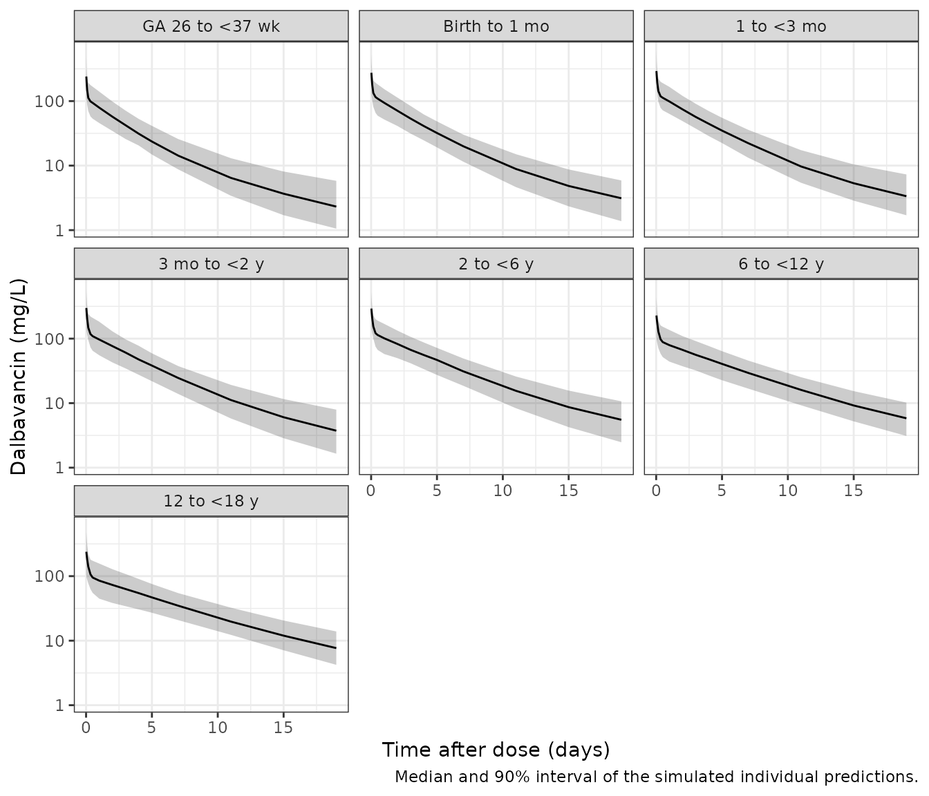
PKNCA validation against Table 1
Table 1 of the paper reports simulated Cmax, AUC0-inf and AUC0-120h
by age group. ncaComparisonTable() pools the per-subject
NCA by median, so the comparison uses the Table 1 medians.
nca_conc <- sim |>
  filter(!is.na(Cc)) |>
  select(id, group, time, Cc)
nca_conc <- bind_rows(
  nca_conc,
  nca_conc |> distinct(id, group) |> mutate(time = 0, Cc = 0)
) |>
  distinct(id, group, time, .keep_all = TRUE) |>
  arrange(id, time)
nca_dose <- dose_rows |> select(id, group, time, amt)

conc_obj <- PKNCA::PKNCAconc(nca_conc, Cc ~ time | group + id)
dose_obj <- PKNCA::PKNCAdose(nca_dose, amt ~ time | group + id)
intervals <- data.frame(
  start = c(0, 0), end = c(Inf, 120),
  cmax = c(TRUE, FALSE), aucinf.obs = c(TRUE, FALSE), auclast = c(FALSE, TRUE)
)
nca_res <- PKNCA::pk.nca(PKNCA::PKNCAdata(conc_obj, dose_obj, intervals = intervals))

published_table1 <- tibble::tribble(
  ~group,             ~cmax, ~aucinf.obs, ~auclast,
  "GA 26 to <37 wk",  220,   13600,       6480,
  "Birth to 1 mo",    283,   14800,       8710,
  "1 to <3 mo",       289,   15300,       8790,
  "3 mo to <2 y",     288,   16200,       9070,
  "2 to <6 y",        282,   19500,       9730,
  "6 to <12 y",       239,   17900,       8530,
  "12 to <18 y",      233,   19900,       8670
) |>
  mutate(group = factor(group, levels = group_levels))

cmp_nca <- nlmixr2lib::ncaComparisonTable(
  simulated = nca_res,
  reference = published_table1,
  by = "group",
  units = c(cmax = "ug/mL", aucinf.obs = "ug*h/mL", auclast = "ug*h/mL"),
  tolerance_pct = 20
)
knitr::kable(
  cmp_nca,
  caption = paste("Simulated vs. Carrothers 2023 Table 1 medians. AUClast is AUC0-120h.",
                  "* differs from reference by >20%.")
)| NCA parameter | group | Reference | Simulated | % diff |
|---|---|---|---|---|
| Cmax (ug/mL) | GA 26 to <37 wk | 220 | 240 | +9.3% |
| Cmax (ug/mL) | Birth to 1 mo | 283 | 274 | -3.1% |
| Cmax (ug/mL) | 1 to <3 mo | 289 | 292 | +1.0% |
| Cmax (ug/mL) | 3 mo to <2 y | 288 | 298 | +3.5% |
| Cmax (ug/mL) | 2 to <6 y | 282 | 292 | +3.5% |
| Cmax (ug/mL) | 6 to <12 y | 239 | 228 | -4.6% |
| Cmax (ug/mL) | 12 to <18 y | 233 | 239 | +2.4% |
| AUC0-∞ (obs) (ug*h/mL) | GA 26 to <37 wk | 13600 | 10000 | -26.2%* |
| AUC0-∞ (obs) (ug*h/mL) | Birth to 1 mo | 14800 | 12800 | -13.7% |
| AUC0-∞ (obs) (ug*h/mL) | 1 to <3 mo | 15300 | 13800 | -10.0% |
| AUC0-∞ (obs) (ug*h/mL) | 3 mo to <2 y | 16200 | 14700 | -9.3% |
| AUC0-∞ (obs) (ug*h/mL) | 2 to <6 y | 19500 | 17800 | -8.8% |
| AUC0-∞ (obs) (ug*h/mL) | 6 to <12 y | 17900 | 16000 | -10.8% |
| AUC0-∞ (obs) (ug*h/mL) | 12 to <18 y | 19900 | 18900 | -4.8% |
| AUClast (ug*h/mL) | GA 26 to <37 wk | 6480 | 6800 | +5.0% |
| AUClast (ug*h/mL) | Birth to 1 mo | 8710 | 8390 | -3.7% |
| AUClast (ug*h/mL) | 1 to <3 mo | 8790 | 8780 | -0.1% |
| AUClast (ug*h/mL) | 3 mo to <2 y | 9070 | 9080 | +0.1% |
| AUClast (ug*h/mL) | 2 to <6 y | 9730 | 9800 | +0.7% |
| AUClast (ug*h/mL) | 6 to <12 y | 8530 | 7990 | -6.4% |
| AUClast (ug*h/mL) | 12 to <18 y | 8670 | 8880 | +2.4% |
nca_by_subject <- as.data.frame(nca_res) |>
  filter(PPTESTCD %in% c("cmax", "aucinf.obs", "auclast")) |>
  group_by(group, PPTESTCD) |>
  summarise(sim = median(PPORRES), .groups = "drop") |>
  left_join(
    published_table1 |>
      tidyr::pivot_longer(-group, names_to = "PPTESTCD", values_to = "ref"),
    by = c("group", "PPTESTCD")
  ) |>
  mutate(pct_diff = 100 * (sim / ref - 1))
term_and_older <- nca_by_subject |> filter(group != "GA 26 to <37 wk")

# Across two cohort draws the per-group Cmax / AUC0-120h differences stayed
# within -6.4% to +7.3% and the AUC0-inf differences within -15.4% to -4.8%
# (median about -10%); the bounds below sit outside that range.
stopifnot(
  # Cmax and AUC0-120h are set by the volumes and the albumin effect on F1; a
  # mis-transcribed volume, dose or albumin form moves every group together.
  abs(median(term_and_older$pct_diff[term_and_older$PPTESTCD != "aucinf.obs"])) < 10,
  all(abs(term_and_older$pct_diff[term_and_older$PPTESTCD != "aucinf.obs"]) < 20),
  # AUC0-inf runs about 10% below Table 1 (see Assumptions); a CL error of the
  # size of a mis-transcribed theta1 or allometric exponent would exceed this.
  abs(median(term_and_older$pct_diff[term_and_older$PPTESTCD == "aucinf.obs"])) < 20
)
For the six term-born groups, Cmax and AUC0-120h match the Table 1 medians within about 10%. AUC0-inf runs about 10-13% below Table 1. The preterm group differs more, because its cohort (birth weight and albumin by gestational age) can only be approximated here (see Assumptions).
Albumin effect form
Neither the paper nor the FDA review prints the functional form of
the albumin effect on F1. The spread of the simulated AUC0-inf in Table
1 separates the two usual candidates. In the birth-to-1-month group the
paper reports AUC0-inf mean (SD) 15,800 (5200), a CV of 33%. That is
about the CV that the 32.8% IIV on CL gives on its own. Under the
paper’s uniform 1.9-5.3 g/dL albumin draw, a power effect adds little to
that spread. A linear effect 1 + 0.385 (ALB - 4.4) would
push F1 close to zero at the lowest albumin values and more than double
the spread.
alb <- seq(1.9, 5.3, length.out = 1000)
f_power <- (alb / 4.4)^0.385
f_linear <- 1 + 0.385 * (alb - 4.4)
data.frame(
  Form = c("Power (used)", "Linear"),
  `F1 range` = c(sprintf("%.2f-%.2f", min(f_power), max(f_power)),
                 sprintf("%.2f-%.2f", min(f_linear), max(f_linear))),
  `CV of F1 (%)` = c(100 * sd(f_power) / mean(f_power), 100 * sd(f_linear) / mean(f_linear)),
  check.names = FALSE
) |>
knitr::kable(digits = 1, caption = "Relative bioavailability F1 over the simulated albumin range.")| Form | F1 range | CV of F1 (%) |
|---|---|---|
| Power (used) | 0.72-1.07 | 10.9 |
| Linear | 0.04-1.35 | 54.7 |
Figure 3: AUC0-120h by age group
nca_auc120 <- as.data.frame(nca_res) |>
  filter(PPTESTCD == "auclast")
ggplot(nca_auc120, aes(group, PPORRES)) +
  geom_boxplot() +
  geom_hline(yintercept = 10400, linetype = "dashed") +
  labs(x = NULL, y = "AUC0-120h (ug*h/mL)",
       caption = paste("Replicates Figure 3 of Carrothers 2023. Dashed line: Table 1 median",
                       "AUC0-120h for adults given 1500 mg (10,400 ug*h/mL).")) +
  theme_bw() +
  theme(axis.text.x = element_text(angle = 30, hjust = 1))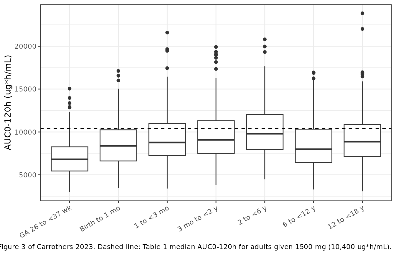
Figure 2: target attainment
The paper defines the daily average free exposure as fAUC0-120h / 5 with fu = 0.07, and uses the S. aureus murine-thigh targets fAUC/MIC = 27.1 (stasis), 53.3 (1-log kill) and 111.1 (2-log kill). Figure 2 shows the 2-log-kill attainment; the Results report PTA of at least 94% up to MIC 2 mg/L for stasis and up to 0.5 mg/L for 2-log kill.
pta <- nca_auc120 |>
  mutate(fauc_avg = 0.07 * PPORRES / 5) |>
  tidyr::crossing(
    target = c(27.1, 53.3, 111.1),
    mic = c(0.0625, 0.125, 0.25, 0.5, 1, 2, 4)
  ) |>
  group_by(group, target, mic) |>
  summarise(pta = 100 * mean(fauc_avg / mic >= target), .groups = "drop")

ggplot(pta |> filter(target == 111.1), aes(mic, pta, colour = group)) +
  geom_line() +
  geom_point() +
  scale_x_log10(breaks = c(0.0625, 0.125, 0.25, 0.5, 1, 2, 4)) +
  labs(x = "MIC (mg/L)", y = "PTA, 2-log kill (%)", colour = "Age group",
       caption = "Replicates the target-attainment curves of Figure 2 of Carrothers 2023.") +
  theme_bw()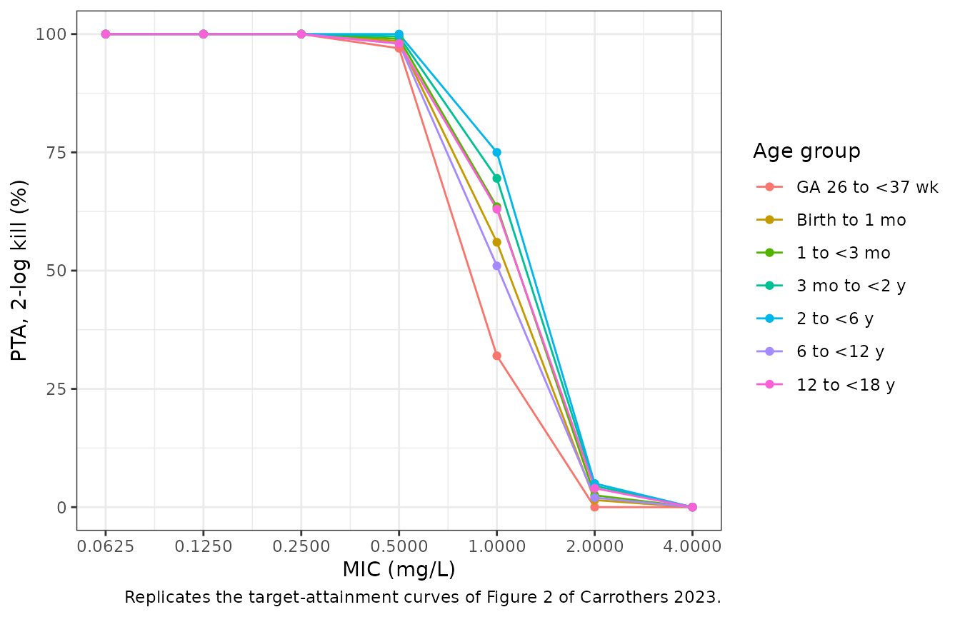
pta |>
  filter((target == 27.1 & mic == 2) | (target == 111.1 & mic == 0.5)) |>
  mutate(target = ifelse(target == 27.1, "Stasis, MIC 2 mg/L", "2-log kill, MIC 0.5 mg/L")) |>
  tidyr::pivot_wider(names_from = target, values_from = pta) |>
  select(-mic) |>
  group_by(group) |>
  summarise(across(everything(), ~ max(.x, na.rm = TRUE)), .groups = "drop") |>
  dplyr::rename(`Age group` = group) |>
knitr::kable(digits = 1, caption = "Simulated PTA (%) at the MICs quoted in the Results (paper: at least 94%).")| Age group | Stasis, MIC 2 mg/L | 2-log kill, MIC 0.5 mg/L |
|---|---|---|
| GA 26 to <37 wk | 97.5 | 97.0 |
| Birth to 1 mo | 99.0 | 98.5 |
| 1 to <3 mo | 99.5 | 99.0 |
| 3 mo to <2 y | 99.5 | 99.5 |
| 2 to <6 y | 100.0 | 100.0 |
| 6 to <12 y | 98.0 | 98.0 |
| 12 to <18 y | 98.0 | 98.0 |
Assumptions and deviations
-
Covariate functional forms. Neither the paper, its
supplement nor the FDA review prints the covariate equations. The model
uses power forms centred on medians:
F1 = (ALB/4.4)^0.385, and(EGFR/74.06)^0.167(age under 2 years) or(CLCRN/100.88)^0.0681(age 2 years and over) on CL. The power form for albumin matches the Table 1 AUC spread, and a linear form does not (see ‘Albumin effect form’). The renal exponents are small enough that a linear form normalised by the reference would behave almost the same. - Centring values. The albumin centring value 4.4 g/dL is the pooled median of the analysis population (FDA review Table 29). The renal references 74.06 and 100.88 mL/min/1.73 m^2 are the age-stratum medians the FDA reviewer used when re-running the model. The reviewer reports that those runs changed the structural estimates by less than 2.3%. The sponsor’s own centring values are not published.
-
theta7. SDC 2 numbers its parameters theta1-theta6
and theta8-theta10. The FDA review states that albumin was
‘parameterized via F (fixed to 1)’. The missing theta7 is taken to be
that fixed typical F1 (
lfcentral). -
Maturation eGFR units. The paper describes the
under-2-years eGFR as ‘a sigmoidal function based on PMA’, and its
preterm simulations derived no height or body surface area. The model
therefore takes the Rhodin maturation term per 70 kg,
121.2 * PMA^3.4 / (47.7^3.4 + PMA^3.4), with size carried by the allometric weight term on CL. The Rhodin constants are those of the theoretical-allometry fit in the Rhodin 2009 abstract. Because the exponent is 0.167, a 20% error in this descriptor changes CL by about 3%. - AUC0-inf about 10% below Table 1. Cmax and AUC0-120h, which depend on the volumes and F1, reproduce Table 1. AUC0-inf, which depends on CL, runs 10-13% low in the term-born groups. The likely causes are the unpublished renal and albumin centring values and the paper’s own AUC0-inf method, which is not described. No parameter was adjusted.
- Cohort. Weight and height for children aged 2 years and over use approximate sex-averaged growth medians with log-normal spread, not the NHANES-correlated, Box-Cox-transformed WHO/CDC draws of the paper. AUC scales with WT^0.25 under mg/kg dosing, so this matters little. For preterm neonates, birth weight by gestational age approximates the Olsen 2010 intrauterine curves. Albumin rises linearly from 2.0 g/dL at 28 weeks to 3.0 g/dL at term, the published values the FDA review cites (Reading and Fleetwood 1990), with 15% log-normal spread. This replaces the paper’s unpublished sigmoidal albumin model. The preterm row of Table 1 is shown for reference and not asserted on.
-
Residual error. Simulations use
STUDY_PHASE3 = 0(phase 1 residual SD). The NCA uses individual predictions (Cc), so the residual error does not enter Table 1 comparisons. -
Adults. The adult column of Table 1 (1500 mg) comes
from the adult model (
Carrothers_2020_dalbavancin) and is not re-simulated here; only its median AUC0-120h is drawn as a reference line in Figure 3.