Model and source
- Citation: Gu F, Tang K, Zhang C, Hu M, Sun J, Yu X, Tian M, Zhang C, Chen Y. Population pharmacokinetic analysis of rivaroxaban in healthy volunteers and patients with radiofrequency ablation of non-valvular atrial fibrillation in China. Front Pharmacol. 2025;16:1562259. doi:10.3389/fphar.2025.1562259
- Description: Two-compartment oral population PK model with first-order absorption, an absorption lag time, and dose-level-dependent relative bioavailability for rivaroxaban in Chinese healthy volunteers and patients treated with radiofrequency ablation for non-valvular atrial fibrillation (Gu 2025)
- Article: https://doi.org/10.3389/fphar.2025.1562259
- Supplementary material (Supplementary Table S1, Sanger-sequencing primers only – no model parameters): https://www.frontiersin.org/articles/10.3389/fphar.2025.1562259/full#supplementary-material
Rivaroxaban is an oral direct factor Xa inhibitor. Gu 2025 pooled a bioequivalence study in healthy Chinese volunteers with a real-world cohort of Chinese patients treated by radiofrequency ablation (RFA) for non-valvular atrial fibrillation (NVAF), and fitted a two-compartment model with first-order absorption, an absorption lag time, dose-level-dependent relative bioavailability, and first-order elimination.
Population
Two studies contributed 1,506 rivaroxaban plasma concentrations from 141 Chinese participants (Gu 2025 Table 1, Results section 3.1):
- Study 1 (CTR20202135) – a single-centre, single-dose, randomized, two-formulation, four-period crossover bioequivalence study in 36 healthy volunteers (32 male / 4 female; age 31.6 +/- 8.9 years, range 18-48; weight 64.2 +/- 5.8 kg; Cockcroft-Gault creatinine clearance 125 +/- 17.8 mL/min, range 91.3-161). Each participant received a single fasted oral 20 mg dose per period, with 18 samples over 48 h; only the reference-formulation (Xarelto) periods contributed the 1,296 modelled concentrations.
- Study 2 (ChiCTR2500095918) – a real-world single-centre study of 105 hospitalized NVAF patients after RFA (60 male / 45 female; age 64.1 +/- 8.4 years, range 34-82; weight 67.4 +/- 11.4 kg, range 42.0-107.0; creatinine clearance 86.7 +/- 24.3 mL/min, range 33.6-158). Patients took 10 mg (n = 2), 15 mg (n = 101), or 20 mg (n = 2) once daily for at least 2 days and contributed one trough (30 min pre-dose) and one peak (2-4 h post-dose) sample each, i.e. 210 concentrations. P-glycoprotein inhibitors (amiodarone, propafenone, felodipine) were co-administered in 56 patients (53.3%) and CYP3A4 inhibitors in 6 (5.7%).
Ten SNPs across CYP3A4, CYP3A5, ABCB1 and ABCG2 were genotyped in every participant (Gu 2025 Table 2). The whole analysis population is Chinese.
The same information is available programmatically via the model’s
population metadata
(readModelDb("Gu_2025_rivaroxaban")()$population).
Source trace
Every ini() entry in
inst/modeldb/specificDrugs/Gu_2025_rivaroxaban.R carries an
in-file comment naming its source location; the table below collects
them.
| Equation / parameter | Value | Source location |
|---|---|---|
lcl (patient reference) |
8.35 L/h | Table 3, row CL/F (L/h), “Clearance of patient” (%RSE
15.8) |
e_dis_healthy_cl |
log(6.48 / 8.35) = -0.2535 | Table 3, “Clearance of healthy volunteer” = 6.48 L/h; Results 3.2
equation legend
TVCL = 6.48 for healthy volunteer, TVCL = 8.35 for patient
|
lvc |
19.7 L | Table 3, row V2/F (L)
|
lka |
0.46 1/h | Table 3, row Ka (1/h)
|
lq |
7.64 L/h | Table 3, row Q/F (L/h)
|
lvp |
71.8 L | Table 3, row V3/F (L)
|
ltlag |
0.168 h | Table 3, row ALAG (h)
|
lfdepot |
fixed(log(1)) | Table 3, row F 15mg = 1 FIX |
e_dose_10mg_fdepot |
fixed(log(1.363)) | Table 3, row F 10mg = 1.363 FIX; Results 3.2 (“fixed
and not estimated in the subsequent models”) |
e_dose_20mg_fdepot |
log(0.537) = -0.6218 | Table 3, row F 20mg (%RSE 15.6) |
e_crcl_cl |
1.53 | Table 3, row CL_crcl; reference 97.7 mL/min from the
Results 3.2 equation |
e_snp_abcb1_rs1045642_hom_cl |
-0.204 | Results 3.2 equation (- AA x 0.204); cross-checks Table
3 row CL_A642 = 0.815 = exp(-0.204) |
etalcl, etalvc, etalka,
etalq, etalvp, etaltlag
|
0.126, 0.350, 0.0773, 0.410, 0.434, 0.602 | Table 3 rows IIV_CL 35.5%, IIV_V2 59.2%,
IIV_Ka 27.8%, IIV_Q 64%, IIV_V3
65.9%, IIV_ALAG 77.6%; variance = (pct/100)^2 |
propSd |
0.263 | Table 3, row delta (proportional residual error) =
26.3% |
CL covariate equation
CL_i = TVCL x exp(1.53 x ln(CRCL_i / 97.7) - AA x 0.204 + eta_CL)
|
n/a | Results section 3.2, printed final-model equation block |
| Two-compartment ODE structure, first-order absorption + lag | n/a | Results section 3.2 first paragraph; Methods section 2.2 |
| Cockcroft-Gault CRCL definition | n/a | Table 1 footnote a |
Note that the display equations do not survive plain-text extraction of the PDF; the covariate equation above was read from the typeset PDF page directly.
Virtual cohort
The original observed data are not public. The cohorts below reproduce the covariate distributions of Gu 2025 Table 1 and the genotype frequencies of Table 2 (AA at ABCB1 rs1045642: 7/36 = 19.4% of healthy volunteers, 20/105 = 19.0% of patients), and use the two studies’ actual dosing and sampling designs.
set.seed(20250529)

n_per_arm <- 100L

# Truncated-normal draw matching a published mean +/- SD and range.
rtrunc_norm <- function(n, mean, sd, lower, upper) {
  out <- numeric(0)
  while (length(out) < n) {
    x <- stats::rnorm(2 * n, mean, sd)
    out <- c(out, x[x >= lower & x <= upper])
  }
  out[seq_len(n)]
}

make_subjects <- function(n, id_offset, healthy, crcl_mean, crcl_sd,
                          crcl_lo, crcl_hi, p_aa) {
  tibble(
    id                      = id_offset + seq_len(n),
    CRCL                    = rtrunc_norm(n, crcl_mean, crcl_sd, crcl_lo, crcl_hi),
    DIS_HEALTHY             = as.numeric(healthy),
    SNP_ABCB1_RS1045642_HOM = stats::rbinom(n, 1L, p_aa)
  )
}

# Study 1: 36 healthy volunteers, single 20 mg oral dose, sampled to 48 h.
hv_subj <- make_subjects(
  n_per_arm, id_offset = 0L, healthy = TRUE,
  crcl_mean = 125, crcl_sd = 17.8, crcl_lo = 91.3, crcl_hi = 161, p_aa = 7 / 36
)
hv_times <- c(0, 0.25, 0.5, 0.75, 1, 1.5, 2, 2.5, 3, 3.5, 4, 5, 6, 8, 10,
              12, 14, 18, 24, 30, 36, 42, 48)

# Study 2: NVAF patients, 15 mg once daily; the trough / peak samples were drawn
# after at least 2 days of dosing, so the profile below is day 5 (steady state).
pt_subj <- make_subjects(
  n_per_arm, id_offset = 1000L, healthy = FALSE,
  crcl_mean = 86.7, crcl_sd = 24.3, crcl_lo = 33.6, crcl_hi = 158, p_aa = 20 / 105
)
pt_dose_times <- seq(0, 96, by = 24)
pt_times <- 96 + c(0, 0.5, 1, 1.5, 2, 2.5, 3, 4, 5, 6, 8, 10, 12, 16, 20, 24)

build_events <- function(subj, dose_mg, dose_times, obs_times, cohort,
                         dose_10mg = 0, dose_20mg = 0) {
  doses <- subj |>
    tidyr::crossing(time = dose_times) |>
    mutate(amt = dose_mg, evid = 1L, cmt = "depot")
  obs <- subj |>
    tidyr::crossing(time = obs_times) |>
    mutate(amt = NA_real_, evid = 0L, cmt = "central")
  bind_rows(doses, obs) |>
    mutate(
      DOSE_10MG = dose_10mg,
      DOSE_20MG = dose_20mg,
      cohort    = cohort
    ) |>
    arrange(id, time, desc(evid)) |>
    as.data.frame()
}

events <- bind_rows(
  build_events(hv_subj, 20, 0, hv_times, "Healthy volunteers, 20 mg single dose",
               dose_20mg = 1),
  build_events(pt_subj, 15, pt_dose_times, pt_times,
               "NVAF patients, 15 mg once daily (day 5)")
)

stopifnot(!anyDuplicated(events[events$evid == 0, c("id", "time")]))
c(subjects = dplyr::n_distinct(events$id), rows = nrow(events))
#> subjects     rows
#>      200     4500
Simulation
mod <- readModelDb("Gu_2025_rivaroxaban")

sim <- rxode2::rxSolve(
  mod, events = events,
  keep = c("cohort", "CRCL", "DIS_HEALTHY", "SNP_ABCB1_RS1045642_HOM")
) |>
  as.data.frame()
#> ℹ parameter labels from comments will be replaced by 'label()'

# rxSolve silently drops subjects whose event records are unusable; assert.
stopifnot(dplyr::n_distinct(sim$id) == 2L * n_per_arm)
Replicate published figures
Figure 2 – concentration-time profiles by cohort
Gu 2025 Figure 2 is a prediction-corrected VPC with the median and 2.5th / 97.5th percentiles, on a log concentration axis: 0-48 h after the single 20 mg dose for healthy volunteers, and 0-24 h after dose for the sparsely sampled patients. The panels below show the same summary statistics from the packaged model.
vpc <- sim |>
  filter(!is.na(Cc)) |>
  mutate(tad = ifelse(cohort == "NVAF patients, 15 mg once daily (day 5)",
                      time - 96, time)) |>
  group_by(cohort, tad) |>
  summarise(
    lo  = quantile(Cc, 0.025),
    mid = quantile(Cc, 0.5),
    hi  = quantile(Cc, 0.975),
    .groups = "drop"
  )

ggplot(vpc, aes(tad, mid)) +
  geom_ribbon(aes(ymin = lo, ymax = hi), alpha = 0.25) +
  geom_line() +
  facet_wrap(~cohort, scales = "free_x") +
  scale_y_log10() +
  labs(x = "Time after dose (h)", y = "Rivaroxaban concentration (ng/mL)",
       caption = "Replicates Figure 2 of Gu 2025 (median and 2.5th-97.5th percentiles).")
#> Warning in scale_y_log10(): log-10 transformation introduced infinite values.
#> log-10 transformation introduced infinite values.
#> log-10 transformation introduced infinite values.
#> log-10 transformation introduced infinite values.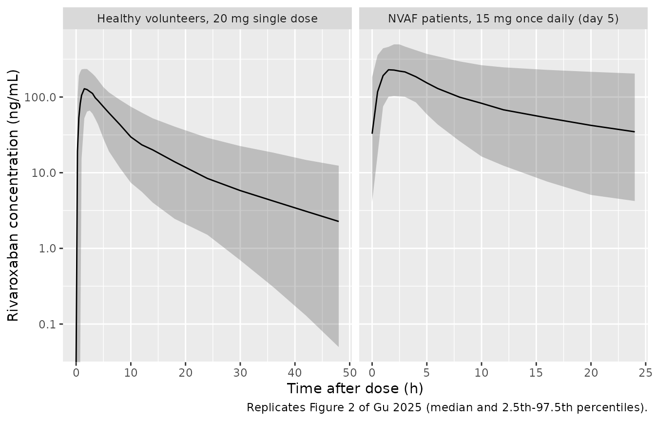
The simulated healthy-volunteer median peaks near 2 h and then falls away faster than the observed median in Gu 2025 Figure 2. The block below quantifies that: the observed median of the healthy-volunteer panel was digitised against the figure’s own log gridlines (1, 10, 100, 1000 ng/mL) and time axis, and is compared with the typical-value profile evaluated at two creatinine clearances – the cohort mean of 125 mL/min (Table 1), and the covariate reference of 97.7 mL/min at which the CRCL term equals 1 and CL/F is exactly the 6.48 L/h that Table 3 reports as the healthy-volunteer typical clearance.
hv_scen <- tibble::tibble(id = 1:2, CRCL = c(125, 97.7))
hv_t <- c(seq(0, 6, by = 0.05), seq(6.25, 48, by = 0.25))

hv_events <- bind_rows(
  hv_scen |> mutate(time = 0, amt = 20, evid = 1L, cmt = "depot"),
  hv_scen |> tidyr::crossing(time = hv_t) |>
    mutate(amt = NA_real_, evid = 0L, cmt = "central")
) |>
  mutate(DIS_HEALTHY = 1, SNP_ABCB1_RS1045642_HOM = 0,
         DOSE_10MG = 0, DOSE_20MG = 1) |>
  arrange(id, time, desc(evid)) |>
  as.data.frame()

hv_typ <- rxode2::rxSolve(rxode2::zeroRe(mod), events = hv_events, omega = NA,
                          keep = "CRCL") |>
  as.data.frame()
#> ℹ parameter labels from comments will be replaced by 'label()'
#> Warning: multi-subject simulation without without 'omega'
hv_typ <- hv_typ[, !duplicated(names(hv_typ))]
stopifnot(dplyr::n_distinct(hv_typ$id) == 2L)

digitised <- tibble::tribble(
  ~tad, ~observed_median,
  2.8,  153,
  14,   24,
  24,   17,
  36,   8.2,
  48,   4.7
)

hv_lab <- function(crcl) {
  ifelse(crcl > 100, "CL/F at CRCL 125 (cohort mean)",
         "CL/F at CRCL 97.7 (covariate reference)")
}

hv_peak <- hv_typ |>
  group_by(crcl_label = hv_lab(CRCL)) |>
  summarise(tad = 2.8, Cc = max(Cc), .groups = "drop")

bind_rows(
  hv_peak,
  hv_typ |>
    filter(time %in% c(14, 24, 36, 48)) |>
    transmute(crcl_label = hv_lab(CRCL), tad = time, Cc)
) |>
  tidyr::pivot_wider(names_from = crcl_label, values_from = Cc) |>
  left_join(digitised, by = "tad") |>
  mutate(across(where(is.numeric), ~ round(.x, 1))) |>
  rename(
    "Time after dose (h)"                      = tad,
    "Gu 2025 Figure 2 observed median (ng/mL)" = observed_median
  ) |>
knitr::kable(caption = "Healthy-volunteer typical-value profile at two creatinine clearances vs the observed median digitised from Gu 2025 Figure 2. The first row compares the peak of each simulated curve (Tmax 1.8-2.0 h) with the peak of the published median (about 2.8 h).")| Time after dose (h) | CL/F at CRCL 125 (cohort mean) | CL/F at CRCL 97.7 (covariate reference) | Gu 2025 Figure 2 observed median (ng/mL) |
|---|---|---|---|
| 2.8 | 144.1 | 162.2 | 153.0 |
| 14.0 | 17.8 | 28.3 | 24.0 |
| 24.0 | 9.7 | 17.3 | 17.0 |
| 36.0 | 5.0 | 10.1 | 8.2 |
| 48.0 | 2.6 | 5.9 | 4.7 |
At the covariate reference the model tracks the published median closely (within about 25% at every time, and within 5% at 2.8 and 24 h). At the cohort’s actual creatinine clearance the printed exponent of 1.53 raises CL/F from 6.48 to 9.45 L/h and the predicted terminal concentrations fall to about half of the published median. This is the first of three internal inconsistencies in Gu 2025 that all point the same way; see “Assumptions and deviations”.
Figure 3 – covariate effects on AUC(0-inf)
Gu 2025 Figure 3 is a forest plot of AUC(0-inf) geometric-mean ratios
computed as dose / CL from the post hoc
individual clearances of the 105 patients, all evaluated at a
15 mg dose (Methods section 2.4): 1.11 for mild and 1.58 for moderate
renal impairment versus normal renal function, and 1.25 for the AA
genotype of ABCB1 rs1045642 versus the other genotypes.
The genotype contrast is reproducible from the printed covariate equation because it is a single multiplicative factor. The renal contrasts are not: the paper does not publish the creatinine clearance of each renal subgroup, and the typical-value prediction from the exponent 1.53 is far steeper than the published ratios (see “Assumptions and deviations”).
# Typical-value clearance from the printed Gu 2025 covariate equation.
cl_typical <- function(crcl, aa = 0, healthy = 0) {
  8.35 * (crcl / 97.7)^1.53 * exp(-0.204 * aa) * exp(log(6.48 / 8.35) * healthy)
}

# Genotype contrast: AUC ratio is the inverse clearance ratio at fixed CRCL.
geno_ratio <- cl_typical(97.7, aa = 0) / cl_typical(97.7, aa = 1)

# Renal contrast at the midpoints of the usual clinical bands, and the CRCL
# ratio that the published AUC ratios imply under the exponent 1.53.
renal <- tibble::tribble(
  ~group,                ~crcl_midpoint, ~published_ratio,
  "Normal (>= 90)",      105,            1.00,
  "Mild (60-89)",        75,             1.11,
  "Moderate (30-59)",    45,             1.58
) |>
  mutate(
    model_ratio  = cl_typical(105) / cl_typical(crcl_midpoint),
    implied_crcl = 105 / published_ratio^(1 / 1.53)
  )

renal |>
  mutate(across(c(model_ratio, implied_crcl), ~ round(.x, 2))) |>
  rename(
    "Renal group (mL/min)"                      = group,
    "Assumed group CRCL (mL/min)"               = crcl_midpoint,
    "Gu 2025 Figure 3 AUC ratio"                = published_ratio,
    "Typical-value AUC ratio from the equation" = model_ratio,
    "CRCL implied by the published ratio"       = implied_crcl
  ) |>
knitr::kable(caption = "Gu 2025 Figure 3 renal subgroups vs the typical-value prediction of the printed CL equation.")| Renal group (mL/min) | Assumed group CRCL (mL/min) | Gu 2025 Figure 3 AUC ratio | Typical-value AUC ratio from the equation | CRCL implied by the published ratio |
|---|---|---|---|---|
| Normal (>= 90) | 105 | 1.00 | 1.00 | 105.00 |
| Mild (60-89) | 75 | 1.11 | 1.67 | 98.08 |
| Moderate (30-59) | 45 | 1.58 | 3.66 | 77.87 |
tibble::tibble(
  contrast   = "ABCB1 rs1045642 AA vs non-AA",
  model      = round(geno_ratio, 3),
  published  = 1.25
) |>
  rename(
    "Contrast"                             = contrast,
    "Typical-value AUC ratio (model)"       = model,
    "Gu 2025 Figure 3 geometric-mean ratio" = published
  ) |>
knitr::kable(caption = "Genotype effect on AUC(0-inf): typical value vs Gu 2025 Figure 3.")| Contrast | Typical-value AUC ratio (model) | Gu 2025 Figure 3 geometric-mean ratio |
|---|---|---|
| ABCB1 rs1045642 AA vs non-AA | 1.226 | 1.25 |
Figure 4 – patient clearance distribution
Gu 2025 Figure 4 plots the post hoc individual clearances of the 105 patients against concomitant CYP3A4 and P-gp inhibitor use. The boxplot medians sit at roughly 9 L/h in every panel. The typical-value clearance implied by the covariate model over the same cohort’s creatinine clearance distribution is lower, because the patients’ mean CRCL of 86.7 mL/min sits below the 97.7 mL/min reference and the exponent 1.53 amplifies that gap.
pt_cl <- pt_subj |>
  mutate(cl_typ = cl_typical(CRCL, aa = SNP_ABCB1_RS1045642_HOM, healthy = 0))

tibble::tibble(
  quantity = c("Typical CL/F at the covariate reference (Table 3)",
               "Median typical CL/F over the simulated patient cohort",
               "Median post hoc individual CL/F read from Gu 2025 Figure 4"),
  value    = c(8.35, round(median(pt_cl$cl_typ), 2), 9.2)
) |>
  rename("Quantity" = quantity, "CL/F (L/h)" = value) |>
knitr::kable(caption = "Patient clearance: covariate-model typical values vs Gu 2025 Figure 4.")| Quantity | CL/F (L/h) |
|---|---|
| Typical CL/F at the covariate reference (Table 3) | 8.35 |
| Median typical CL/F over the simulated patient cohort | 6.63 |
| Median post hoc individual CL/F read from Gu 2025 Figure 4 | 9.20 |
PKNCA validation
The paper reports AUC(0-inf) for the three patient dose levels,
computed as dose / CL at the typical patient clearance (Gu
2025 Discussion). The scenarios below reproduce those conditions
deterministically: a typical NVAF patient (DIS_HEALTHY = 0,
CRCL = 97.7 mL/min, non-AA genotype) receiving a single 10,
15, or 20 mg dose, plus the typical healthy volunteer of Study 1 (20 mg,
CRCL = 125 mL/min).
scenarios <- tibble::tribble(
  ~scenario,                  ~amt, ~healthy, ~crcl, ~d10, ~d20,
  "Patient, 10 mg",           10,   0,        97.7,  1,    0,
  "Patient, 15 mg",           15,   0,        97.7,  0,    0,
  "Patient, 20 mg",           20,   0,        97.7,  0,    1,
  "Healthy volunteer, 20 mg", 20,   1,        125,   0,    1
) |>
  mutate(id = seq_len(n()))

nca_times <- c(seq(0, 6, by = 0.1), seq(6.25, 24, by = 0.25), seq(25, 168, by = 1))

nca_events <- bind_rows(
  scenarios |> mutate(time = 0, evid = 1L, cmt = "depot"),
  scenarios |> select(-amt) |> tidyr::crossing(time = nca_times) |>
    mutate(amt = NA_real_, evid = 0L, cmt = "central")
) |>
  transmute(
    id, time, amt, evid, cmt, scenario,
    CRCL = crcl, DIS_HEALTHY = healthy,
    SNP_ABCB1_RS1045642_HOM = 0,
    DOSE_10MG = d10, DOSE_20MG = d20
  ) |>
  arrange(id, time, desc(evid)) |>
  as.data.frame()

sim_typical <- rxode2::rxSolve(
  rxode2::zeroRe(mod), events = nca_events, omega = NA,
  keep = c("scenario", "CRCL", "DIS_HEALTHY", "DOSE_10MG", "DOSE_20MG")
) |>
  as.data.frame()
#> ℹ parameter labels from comments will be replaced by 'label()'
#> Warning: multi-subject simulation without without 'omega'

stopifnot(dplyr::n_distinct(sim_typical$id) == nrow(scenarios))
stopifnot(all(sim_typical$Cc >= 0, na.rm = TRUE))
sim_nca <- sim_typical |>
  filter(!is.na(Cc)) |>
  select(id, time, Cc, scenario)

# Guarantee a time = 0 record per subject (Cc = 0 pre-dose, extravascular).
sim_nca <- bind_rows(
  sim_nca,
  sim_nca |> distinct(id, scenario) |> mutate(time = 0, Cc = 0)
) |>
  distinct(id, scenario, time, .keep_all = TRUE) |>
  arrange(id, scenario, time)

conc_obj <- PKNCA::PKNCAconc(sim_nca, Cc ~ time | scenario + id)

dose_df <- nca_events |>
  filter(evid == 1L) |>
  select(id, time, amt, scenario)
dose_obj <- PKNCA::PKNCAdose(dose_df, amt ~ time | scenario + id)

intervals <- data.frame(
  start      = 0,
  end        = Inf,
  cmax       = TRUE,
  tmax       = TRUE,
  aucinf.obs = TRUE,
  half.life  = TRUE
)

nca_res <- PKNCA::pk.nca(PKNCA::PKNCAdata(conc_obj, dose_obj, intervals = intervals))
Structural identity: AUC(0-inf) = F x dose / CL
For a linear model the NCA AUC(0-inf) must equal the relative bioavailability times dose divided by apparent clearance. This is a per-scenario identity, so it is asserted exactly rather than compared by eye.
f_rel <- function(d10, d20) 1.363^d10 * 0.537^d20

identity_tbl <- scenarios |>
  mutate(
    cl_pred    = cl_typical(crcl, aa = 0, healthy = healthy),
    auc_theory = f_rel(d10, d20) * amt / cl_pred * 1000
  ) |>
  left_join(
    as.data.frame(nca_res) |>
      filter(PPTESTCD == "aucinf.obs") |>
      select(scenario, auc_nca = PPORRES),
    by = "scenario"
  ) |>
  mutate(pct_diff = 100 * (auc_nca - auc_theory) / auc_theory)

stopifnot(max(abs(identity_tbl$pct_diff)) < 1)

identity_tbl |>
  transmute(
    scenario,
    cl_pred    = round(cl_pred, 2),
    auc_theory = round(auc_theory),
    auc_nca    = round(auc_nca),
    pct_diff   = round(pct_diff, 3)
  ) |>
  rename(
    "Scenario"                        = scenario,
    "CL/F (L/h)"                      = cl_pred,
    "F x dose / CL (ng*h/mL)"         = auc_theory,
    "PKNCA AUC(0-inf) (ng*h/mL)"      = auc_nca,
    "Difference (%)"                  = pct_diff
  ) |>
knitr::kable(caption = "Per-scenario AUC identity check (all within 1%).")| Scenario | CL/F (L/h) | F x dose / CL (ng*h/mL) | PKNCA AUC(0-inf) (ng*h/mL) | Difference (%) |
|---|---|---|---|---|
| Patient, 10 mg | 8.35 | 1632 | 1632 | 0.006 |
| Patient, 15 mg | 8.35 | 1796 | 1797 | 0.006 |
| Patient, 20 mg | 8.35 | 1286 | 1286 | 0.006 |
| Healthy volunteer, 20 mg | 9.45 | 1137 | 1137 | 0.006 |
Comparison against the published exposures
Gu 2025 reports AUC(0-inf) of 1,198 / 1,796 / 2,395 ng*h/mL for the
10 / 15 / 20 mg patient doses (Discussion), obtained from the formula
dose / CL with CL = 8.35 L/h. That formula omits the
dose-level relative bioavailability the same paper estimates (1.363 at
10 mg, 0.537 at 20 mg), so the packaged model agrees exactly at the 15
mg reference dose – where F is fixed to 1 by definition and the paper’s
own covariate analysis was anchored (“all subjects receiving a
consistent dose of 15 mg”, Methods 2.4) – and differs at the other two
dose levels by exactly the relative-bioavailability factor.
published <- tibble::tribble(
  ~scenario,        ~aucinf.obs,
  "Patient, 10 mg", 1198,
  "Patient, 15 mg", 1796,
  "Patient, 20 mg", 2395
)

cmp <- nlmixr2lib::ncaComparisonTable(
  simulated     = nca_res,
  reference     = published,
  by            = "scenario",
  params        = "aucinf.obs",
  units         = c(aucinf.obs = "ng*h/mL"),
  tolerance_pct = 20
)

knitr::kable(
  cmp,
  caption = "Simulated vs published AUC(0-inf). * differs from the published value by >20%; the 10 mg and 20 mg rows differ by exactly the relative bioavailability factor (1.363 and 0.537) that the paper's dose/CL formula omits."
)| NCA parameter | scenario | Reference | Simulated | % diff |
|---|---|---|---|---|
| AUC0-∞ (obs) (ng*h/mL) | Patient, 10 mg | 1200 | 1630 | +36.3%* |
| AUC0-∞ (obs) (ng*h/mL) | Patient, 15 mg | 1800 | 1800 | +0.0% |
| AUC0-∞ (obs) (ng*h/mL) | Patient, 20 mg | 2400 | 1290 | -46.3%* |
as.data.frame(nca_res) |>
  filter(PPTESTCD %in% c("cmax", "tmax", "half.life")) |>
  select(scenario, PPTESTCD, PPORRES) |>
  tidyr::pivot_wider(names_from = PPTESTCD, values_from = PPORRES) |>
  mutate(across(where(is.numeric), ~ round(.x, 2))) |>
  rename(
    "Scenario"                 = scenario,
    "Cmax (ng/mL)"             = cmax,
    "Tmax (h)"                 = tmax,
    "Terminal half-life (h)"   = half.life
  ) |>
knitr::kable(caption = "Typical-value NCA summary from the packaged model.")| Scenario | Cmax (ng/mL) | Tmax (h) | Terminal half-life (h) |
|---|---|---|---|
| Healthy volunteer, 20 mg | 144.15 | 1.8 | 12.42 |
| Patient, 10 mg | 190.66 | 1.9 | 13.25 |
| Patient, 15 mg | 209.82 | 1.9 | 13.25 |
| Patient, 20 mg | 150.23 | 1.9 | 13.25 |
The typical-value Cmax of the 20 mg healthy volunteer (144 ng/mL at 1.8 h) is close to the peak of the observed median in Gu 2025 Figure 2 (about 153 ng/mL near 2.8 h), and the terminal half-life sits just above the 5-13 h range quoted for rivaroxaban in the Gu 2025 Introduction.
Assumptions and deviations
IIV reporting scale. Gu 2025 Table 3 reports each IIV as a bare percentage with no stated convention. The percentages are read as
omega = pct / 100(soomega^2 = (pct/100)^2) rather than as lognormal CVs (omega^2 = log(1 + CV^2)), for two reasons: the same “(%)” column of the same table reports the proportional residual error as 26.3%, where the only sensible computation issqrt(sigma^2) x 100; and propagating each row’s own %RSE on the printed percentage scale reproduces the published bootstrap intervals better than the lognormal-CV transform does (for the largest IIV,IIV_ALAG77.6% with %RSE 13.7, the printed-scale propagation gives 56.8-98.4 against a published bootstrap interval of 52.2-95.4, versus 55.4-108.7 under the lognormal-CV reading). The choice changes omega by at most 12% (onIIV_ALAG) and by 3% onIIV_CL.-
The published creatinine-clearance exponent of 1.53 is not consistent with three of the paper’s own figures. The exponent is encoded exactly as published, but users simulating renally-impaired or supranormal-CRCL subjects should know that it produces a much steeper renal gradient than Gu 2025’s own results imply:
- Figure 2 (VPC). The healthy-volunteer cohort has a mean creatinine clearance of 125 mL/min, where the exponent inflates CL/F from 6.48 to 9.45 L/h. The resulting typical profile falls to roughly half the observed median from 24 h onward. Setting the CRCL term to 1 (CL/F = 6.48 L/h, the healthy-volunteer typical of Table 3) reproduces the published median within about 25% at every digitised time point.
- Figure 3 (covariate forest plot). At the midpoints of the conventional renal bands the typical-value AUC ratios are about 1.7 (mild) and 3.7 (moderate) versus normal renal function, against the published 1.11 and 1.58. Inverting the published ratios under the exponent 1.53 implies subgroup creatinine clearances of about 98 and 78 mL/min, which fall in the “normal” and “mild” bands rather than in the mild and moderate bands they are supposed to represent.
- Figure 4 (patient clearance distribution). The post hoc individual clearances of the 105 patients have a median near 9 L/h, whereas the covariate model evaluated over the same cohort’s creatinine clearances gives a typical value near 6.5 L/h.
Checks 1 and 3 pull in opposite directions (the model is too fast for the high-CRCL healthy cohort and too slow for the lower-CRCL patient cohort), which is the signature of a covariate slope steeper than the data support – plausibly because creatinine clearance is strongly confounded with study and age here (healthy volunteers: 31.6 years, 125 mL/min; patients: 64.1 years, 86.7 mL/min). An exponent near 0.5 would reconcile all three figures, but no such value appears anywhere in the paper, so none is used: the value 1.53 is printed twice, in Table 3 (
CL_crcl, %RSE 11.9, bootstrap median 1.53, interval 1-1.97) and in the Results section 3.2 equation, and parameters are never tuned to a validation target. Figures 3 and 4 aggregate post hoc individual clearances (Methods section 2.4), which shrink toward each subject’s own sparse data and can therefore look flatter than the typical value model; that explanation does not cover check 1, which compares against the paper’s own model-simulated VPC band. The paper publishes neither the per-subgroup creatinine clearances nor the individual parameter table needed to settle it, so the discrepancy is documented rather than resolved. Genotype nomenclature. The Gu 2025 Discussion calls the AA stratum of ABCB1 rs1045642 the “wild genotype”, which conflicts with the standard dbSNP orientation (A is the c.3435T variant allele) and with the paper’s own allele frequencies (G = 0.60, A = 0.40 in the patient cohort). The model file encodes the covariate exactly as the printed equation defines it (
AA = 1for the AA genotype, 0 otherwise) under the canonical nameSNP_ABCB1_RS1045642_HOM, and does not depend on the prose label.Residual error. Methods section 2.2 describes a combined proportional plus additive residual model, but Table 3 of the final model reports only the proportional term (26.3%), so only
propSdis encoded.Covariates screened but not retained. Sex, age, height, weight, WBC, RBC, platelets, glucose, creatinine, ALT, AST, calcium, potassium, creatine kinase, and nine of the ten genotyped SNPs were screened and not retained; weight entered the full model on the peripheral volume but was removed in backward elimination and no point estimate is published for it. Concomitant P-gp inhibitor use was associated with lower post hoc clearance (Figure 4, p = 0.046) but was not carried into the final model. All of these are recorded in the model file’s
covariatesDataExcludedlist so the screen is documented without adding unused covariates.Steady-state patient panel. Gu 2025 Figure 2 plots the patient observations against time after dose without stating the dosing day; the patient panel here uses day 5 of 15 mg once daily, consistent with the “minimum of 2 days of rivaroxaban administration” enrollment rule in Methods section 2.1.2.
Virtual cohort. Creatinine clearance is drawn from a normal distribution truncated at the published range, matching the Table 1 mean and SD per study; the ABCB1 rs1045642 AA indicator is drawn as a Bernoulli variable at the Table 2 genotype frequency. Weight, age and sex are not needed by the model (they enter only through the Cockcroft-Gault creatinine clearance, which is simulated directly), so they are not carried in the cohort.
Supplementary material. The Gu 2025 electronic supplementary material (Supplementary Table S1) contains only the Sanger-sequencing primer sequences; it holds no model parameters. No erratum or corrigendum exists for this article (Europe PMC comment/correction list checked 2026-08-16).