Buprenorphine, norbuprenorphine and naloxone sublingual combination (Gu 2023)
Source:vignettes/articles/Gu_2023_buprenorphine_naloxone.Rmd
Gu_2023_buprenorphine_naloxone.RmdModel and source
- Citation: Gu M, Li A, Mak W, Dong F, Xu N, Zhang J, Shi Y, Zheng N, Tang Z, He Q, Ruan C, Guo W, Xiang X, Wang C, Han B, Zhu X (2023). Population pharmacokinetics of buprenorphine and naloxone sublingual combination in Chinese healthy volunteers and patients with opioid use disorder: Model-based dose optimization. Front. Pharmacol. 14:1089862. doi:10.3389/fphar.2023.1089862.
- Buprenorphine model: Parent-metabolite population PK model for sublingual buprenorphine and its metabolite norbuprenorphine after the buprenorphine/naloxone (4:1) sublingual tablet in Chinese male healthy volunteers and patients with opioid use disorder (Gu 2023). Buprenorphine: two-compartment disposition with Savic transit absorption (8 transit compartments fixed, estimated mean transit time) into an absorption compartment emptying at first-order ka; relative bioavailability falls linearly with the number of swallows after dosing (reference 3 swallows). Norbuprenorphine: two-compartment disposition formed from the whole buprenorphine clearance (fraction metabolised fixed to 1, multiplied by 1.98 in the 16 mg dose group). The transit chain is explicit, so the dose (mg buprenorphine) is given to transit1; the absorbed amount carries the factor from the control stream’s Stirling approximation to log(n!). The naloxone component is a separately fitted model (Gu_2023_naloxone).
- Naloxone model: One-compartment population PK model for naloxone after the sublingual buprenorphine/naloxone (4:1) tablet in Chinese male healthy volunteers and patients with opioid use disorder (Gu 2023). First-order absorption (no IIV on ka), bioavailability fixed to 0.01 at the 8 mg dose level with a power effect of dose (exponent -0.36), and combined additive and proportional residual error. The dose is entered as the labelled buprenorphine strength of the combination dose (8 mg for four 2 mg/0.5 mg tablets carrying 2 mg naloxone), as in the published model. The buprenorphine and norbuprenorphine component is a separately fitted model (Gu_2023_buprenorphine).
- Article: https://doi.org/10.3389/fphar.2023.1089862 (open access)
- Supplement: https://www.frontiersin.org/articles/10.3389/fphar.2023.1089862/full#supplementary-material (Tables S1-S3 and the NONMEM control streams of both final models)
Gu et al. analysed buprenorphine (BUP), its metabolite norbuprenorphine (norBUP) and naloxone (NLX) after the sublingual buprenorphine/naloxone 4:1 tablet. Because the two drugs do not interact pharmacokinetically, the authors fitted two separate NONMEM models, and they are packaged here as two files:
-
Gu_2023_buprenorphine– a parent-metabolite model. Buprenorphine has two-compartment disposition and Savic transit absorption (8 transit compartments, fixed) into an absorption compartment emptied at first order. Its relative bioavailability falls by 3.5% per swallow after dosing (centred on 3 swallows). Norbuprenorphine (two compartments) is formed from the whole buprenorphine clearance, with the fraction metabolised fixed to 1 at 4 and 8 mg and multiplied by 1.98 at 16 mg. -
Gu_2023_naloxone– a one-compartment model with first-order absorption, a fixed sublingual bioavailability of 0.01 at the 8 mg dose level and a power effect of dose on that bioavailability.
Dosing. Both models take the dose in mg of
labelled buprenorphine (one tablet = 2 mg buprenorphine + 0.5
mg naloxone). In Gu_2023_buprenorphine the dose goes to
transit1, the first compartment of the transit chain; in
Gu_2023_naloxone it goes to depot, and its
amt is not the naloxone content: an 8 mg
buprenorphine dose carrying 2 mg naloxone is entered as
amt = 8, exactly as in the source data (see Assumptions
and deviations). Both models also need the covariate
DOSE_BPN_SL_MG set to the same per-dose value; the
buprenorphine model also needs NSWALLOWS, the number of
swallows after the dose. Concentrations are returned in ng/mL (the paper
reports ng/L).
Population
46 Han Chinese men took part at Beijing Anding Hospital (Table 1): 34 healthy volunteers received a single dose of 4 mg (n = 12), 8 mg (n = 12) or 16 mg (n = 10) buprenorphine under naltrexone blockade, and 12 patients with opioid use disorder (OUD) took 8 mg once daily for 8 days. Median age was 27.5 years (20-44) and median weight 65.0 kg (53-88). The number of swallows after the dose was recorded only in the single-dose groups: median 3.5 (0-8) at 4 mg, 2 (0-3) at 8 mg and 6.5 (2-12) at 16 mg; it was imputed with 2 in the multiple-dose group. The data comprised 699 buprenorphine, 691 norbuprenorphine and 484 naloxone concentrations. Below-LLOQ data were under 10% for buprenorphine and norbuprenorphine (discarded) and 20.3% / 56.2% (single / multiple dose) for naloxone (M3 method).
The same information is available programmatically via
readModelDb("Gu_2023_buprenorphine")()$population.
Source trace
Every ini() value carries an in-file comment pointing to
its source. The supplementary control streams were used to confirm
structure, and they settle two points the printed tables leave ambiguous
(see Assumptions and deviations).
| Equation / parameter | Value | Source location |
|---|---|---|
lcl (BUP CL/F) |
270 L/h | Table 4 |
lvc (BUP Vc/F) |
377 L | Table 4 |
lvp (BUP Vp/F) |
5879 L | Table 4 |
lq (BUP Q/F) |
404 L/h | Table 4 |
lka |
0.397 1/h | Table 4 |
lmtt |
0.234 h | Table 4 |
lntr |
8 (fixed) | Control stream THETA(6) (8) FIX; Figure 1A |
e_nswallows_fdepot |
-0.035 | Table 4 ‘The effect of NOS on F’; control stream
TVSLDO=DOSE*(1+THETA(8)*(NOS-3))
|
fm |
1 (fixed) | Section 3.1.1; control stream THETA(17) (1) FIX
|
e_dose16_fm |
1.98 | Table 4 ‘Fm increment of 16 mg’; control stream
IF(DOSE.EQ.16) FFACTOR = THETA(18)
|
lcl_norbup |
264 L/h | Control stream TVCLM=THETA(10) (Table 4 row labelled ‘V
C norBUP /Fm’) |
lvc_norbup |
22.2 L | Control stream TVV4=THETA(9) (Table 4 row labelled ‘CL
norBUP /Fm’) |
lvp_norbup |
5170 L | Table 4 |
lq_norbup |
705 L/h | Table 4 |
| BUP IIV (CL, Vc, Vp, Q, MTT) | 33.2, 135.6, 41.4, 49.4, 37.5 %CV | Table 4; omega^2 = (CV/100)^2 (control stream
$OMEGA) |
| norBUP IIV (CL, Vc, Vp, Q) | 50.5, 119.6, 45.1, 56.7 %CV | Table 4 (CL / Vc rows swapped, as above) |
propSd, propSd_norbup
|
0.281, 0.22 | Table 4; additive parts (0) FIX in the control
stream |
NLX lcl, lvc, lka
|
205 L/h, 104 L, 0.585 1/h | Table 3 |
NLX lfdepot
|
0.01 (fixed) | Table 3; control stream THETA(4) 0.01 FIX
|
NLX e_dose_fdepot
|
-0.36 | Table 3; control stream
TVF1 = THETA(4)*(DOSE/8)**THETA(7)
|
| NLX IIV (CL, Vc) | 31.2, 102.5 %CV | Table 3 |
NLX propSd, addSd
|
0.208, 9.24 ng/L | Table 3; control stream
SD = SQRT(THETA(5)**2*IPRED**2 + THETA(6)**2)
|
| Savic transit input | n/a | Control stream $DES DADT(1), with
LNFAC = LOG(2.5066)+(N+0.5)*LOG(N)-N; explicit
9-compartment chain here |
| Parent-metabolite ODEs | n/a | Control stream $DES
DADT(2)-DADT(5)
|
| Concentration scaling | n/a | Control streams CP = A(2)/V2*1000000,
S2=V/1000000 (ng/L; ng/mL here) |
Mass-balance and covariate checks (typical values)
These deterministic checks confirm that the transit chain delivers the dose, that the metabolite is formed from the whole parent clearance, and that the covariate effects have the published size. Each one goes red on a zeroed or doubled input, a wrong clearance or a mis-signed covariate.
# Event table for the parent-metabolite model. Doses go to `transit1`, the
# first compartment of the explicit transit chain. With two declared error
# endpoints every observation row nominates one via `dvid`; both Cc and
# Cc_norbup come back as columns. Covariates follow the event columns.
bup_events <- function(ids, dose_times, dose_amt, obs_times, nswallows) {
  dose_amt <- rep_len(dose_amt, length(dose_times))
  one <- dplyr::bind_rows(
    data.frame(time = dose_times, amt = dose_amt, evid = 1L, cmt = "transit1", dvid = NA_integer_),
    data.frame(time = obs_times, amt = 0, evid = 0L, cmt = NA_character_, dvid = 1L)
  ) |>
    dplyr::arrange(time, dplyr::desc(evid))
  # DOSE_BPN_SL_MG is the most recent dose (only the 16 mg level changes the
  # norbuprenorphine Fm; buprenorphine itself does not depend on it).
  one$DOSE_BPN_SL_MG <- dose_amt[findInterval(one$time, dose_times)]
  ev <- dplyr::bind_rows(lapply(ids, function(i) dplyr::mutate(one, id = i)))
  ev$NSWALLOWS <- rep_len(nswallows, length(ids))[match(ev$id, ids)]
  dplyr::select(ev, id, time, amt, evid, cmt, dvid, DOSE_BPN_SL_MG, NSWALLOWS)
}

# Event table for the one-endpoint naloxone model: observations on `central`.
nlx_events <- function(ids, dose_times, dose_amt, obs_times) {
  dose_amt <- rep_len(dose_amt, length(dose_times))
  one <- dplyr::bind_rows(
    data.frame(time = dose_times, amt = dose_amt, evid = 1L, cmt = "depot"),
    data.frame(time = obs_times, amt = 0, evid = 0L, cmt = "central")
  ) |>
    dplyr::arrange(time, dplyr::desc(evid))
  one$DOSE_BPN_SL_MG <- dose_amt[findInterval(one$time, dose_times)]
  ev <- dplyr::bind_rows(lapply(ids, function(i) dplyr::mutate(one, id = i)))
  dplyr::select(ev, id, time, amt, evid, cmt, DOSE_BPN_SL_MG)
}

trap <- function(t, y) sum(diff(t) * (head(y, -1) + tail(y, -1)) / 2)
mod_bup <- readModelDb("Gu_2023_buprenorphine")
mod_nlx <- readModelDb("Gu_2023_naloxone")
bup_typ <- rxode2::zeroRe(mod_bup)
#> ℹ parameter labels from comments will be replaced by 'label()'
nlx_typ <- rxode2::zeroRe(mod_nlx)
#> ℹ parameter labels from comments will be replaced by 'label()'

# Log-spaced grid to 2000 h: the norbuprenorphine terminal phase is long.
grid <- c(0, 10^seq(-3, log10(2000), length.out = 4000))
# Stirling's approximation to log(8!) in the control stream makes the transit
# input deliver 1.0105 times the bioavailable dose.
stirling <- exp(lgamma(9) - (log(2.5066) + 8.5 * log(8) - 8))

mb <- lapply(c(4, 8, 16), function(d) {
  lapply(c(3, 4), function(nos) {
    ev <- bup_events(1L, 0, d, grid, nos)
    s <- as.data.frame(rxode2::rxSolve(bup_typ, ev, atol = 1e-12, rtol = 1e-10))
    s <- s[!duplicated(s$time), ]
    data.frame(
      dose = d, nos = nos,
      bup_ratio = 270 * trap(s$time, s$Cc) / 1000 / d,
      norbup_ratio = 264 * trap(s$time, s$Cc_norbup) / 1000 / d
    )
  }) |> dplyr::bind_rows()
}) |> dplyr::bind_rows()
#> ℹ omega/sigma items treated as zero: 'etalcl', 'etalvc', 'etalvp', 'etalq', 'etalmtt', 'etalcl_norbup', 'etalvc_norbup', 'etalvp_norbup', 'etalq_norbup'
#> ℹ omega/sigma items treated as zero: 'etalcl', 'etalvc', 'etalvp', 'etalq', 'etalmtt', 'etalcl_norbup', 'etalvc_norbup', 'etalvp_norbup', 'etalq_norbup'
#> ℹ omega/sigma items treated as zero: 'etalcl', 'etalvc', 'etalvp', 'etalq', 'etalmtt', 'etalcl_norbup', 'etalvc_norbup', 'etalvp_norbup', 'etalq_norbup'
#> ℹ omega/sigma items treated as zero: 'etalcl', 'etalvc', 'etalvp', 'etalq', 'etalmtt', 'etalcl_norbup', 'etalvc_norbup', 'etalvp_norbup', 'etalq_norbup'
#> ℹ omega/sigma items treated as zero: 'etalcl', 'etalvc', 'etalvp', 'etalq', 'etalmtt', 'etalcl_norbup', 'etalvc_norbup', 'etalvp_norbup', 'etalq_norbup'
#> ℹ omega/sigma items treated as zero: 'etalcl', 'etalvc', 'etalvp', 'etalq', 'etalmtt', 'etalcl_norbup', 'etalvc_norbup', 'etalvp_norbup', 'etalq_norbup'

mb <- mb |>
  dplyr::mutate(
    f_expected = (1 - 0.035 * (nos - 3)) * stirling,
    fm_expected = ifelse(dose == 16, 1.98, 1)
  )
knitr::kable(mb, digits = 5,
caption = "CL x AUC(0-inf) / dose for buprenorphine and norbuprenorphine (typical values).")| dose | nos | bup_ratio | norbup_ratio | f_expected | fm_expected |
|---|---|---|---|---|---|
| 4 | 3 | 1.01048 | 1.01048 | 1.01048 | 1.00 |
| 4 | 4 | 0.97511 | 0.97511 | 0.97511 | 1.00 |
| 8 | 3 | 1.01048 | 1.01048 | 1.01048 | 1.00 |
| 8 | 4 | 0.97511 | 0.97511 | 0.97511 | 1.00 |
| 16 | 3 | 1.01048 | 2.00075 | 1.01048 | 1.98 |
| 16 | 4 | 0.97511 | 1.93072 | 0.97511 | 1.98 |
stopifnot(
  # CL/F x AUC = F(NOS) x dose x Stirling factor.
  all(abs(mb$bup_ratio / mb$f_expected - 1) < 1e-3),
  # CLm/Fm x AUCm = Fm x F(NOS) x dose x Stirling factor.
  all(abs(mb$norbup_ratio / (mb$f_expected * mb$fm_expected) - 1) < 1e-3)
)

nlx_mb <- lapply(c(4, 8, 16), function(d) {
  ev <- nlx_events(1L, 0, d, grid[grid <= 400])
  s <- as.data.frame(rxode2::rxSolve(nlx_typ, ev, atol = 1e-12, rtol = 1e-10))
  s <- s[!duplicated(s$time), ]
  data.frame(dose = d, ratio = 205 * trap(s$time, s$Cc) / 1000 / d,
             f_expected = 0.01 * (d / 8)^-0.36)
}) |> dplyr::bind_rows()
#> ℹ omega/sigma items treated as zero: 'etalcl', 'etalvc'
#> ℹ omega/sigma items treated as zero: 'etalcl', 'etalvc'
#> ℹ omega/sigma items treated as zero: 'etalcl', 'etalvc'
knitr::kable(nlx_mb, digits = 5,
caption = "Naloxone CL x AUC(0-inf) / dose against F = 0.01 (DOSE/8)^-0.36.")| dose | ratio | f_expected |
|---|---|---|
| 4 | 0.01283 | 0.01283 |
| 8 | 0.01000 | 0.01000 |
| 16 | 0.00779 | 0.00779 |
The 3.5% fall in buprenorphine bioavailability per additional swallow
(Abstract and Section 4.3) is the nos = 4 versus
nos = 3 rows above, and the 1.98-fold higher
norbuprenorphine exposure per unit of parent clearance at 16 mg (Section
4.3) is the 16 mg norbup_ratio.
Virtual cohort
The observed data are not public. Each published dose group is simulated with 200 virtual subjects at the paper’s sampling times (Section 2.4). The number of swallows is set to the Table 1 median of each single-dose group, and to 2 in the multiple-dose group, as the authors imputed it.
n_arm <- 200L
sd_times <- c(0, 0.25, 0.5, 0.75, 1, 1.5, 2, 3, 4, 6, 8, 10, 12, 24, 36, 48, 60, 72)
md_doses <- seq(0, 168, by = 24)
md_times <- c(0, 120, 144, 168 + c(0, 0.25, 0.5, 1, 1.5, 2, 4, 8, 12, 24))

arms <- data.frame(
  treatment = c("4 mg", "8 mg", "16 mg", "8 mg QD x 8 d"),
  dose = c(4, 8, 16, 8),
  nos = c(3.5, 2, 6.5, 2),
  multiple = c(FALSE, FALSE, FALSE, TRUE)
)

build_arm <- function(k, builder) {
  a <- arms[k, ]
  ids <- (k - 1L) * n_arm + seq_len(n_arm)
  dt <- if (a$multiple) md_doses else 0
  ot <- if (a$multiple) md_times else sd_times
  ev <- if (identical(builder, "bup")) {
    bup_events(ids, dt, a$dose, ot, a$nos)
  } else {
    nlx_events(ids, dt, a$dose, ot)
  }
  dplyr::mutate(ev, treatment = a$treatment)
}

ev_bup <- dplyr::bind_rows(lapply(seq_len(nrow(arms)), build_arm, builder = "bup"))
ev_nlx <- dplyr::bind_rows(lapply(seq_len(nrow(arms)), build_arm, builder = "nlx"))
stopifnot(
  !anyDuplicated(unique(ev_bup[, c("id", "time", "evid")])),
  length(unique(ev_bup$id)) == 4L * n_arm
)
Simulation
rxode2::rxSetSeed(20230119)
sim_bup <- rxode2::rxSolve(mod_bup, events = ev_bup, keep = "treatment") |>
  as.data.frame()
#> ℹ parameter labels from comments will be replaced by 'label()'
sim_nlx <- rxode2::rxSolve(mod_nlx, events = ev_nlx, keep = "treatment") |>
  as.data.frame()
#> ℹ parameter labels from comments will be replaced by 'label()'

# The published predictive check summarises simulated observations, so the
# residual error of each model is added here (Tables 3 and 4) and values below
# the assay LLOQ (50 ng/L for BUP and norBUP, 20 ng/L for NLX; Section 2.5)
# are set to zero, which PKNCA treats as below the limit of quantification.
# Cc keeps this observation-scale value; ipred is the noise-free prediction.
set.seed(20230119)
add_ruv <- function(ipred, prop, add = 0, lloq) {
  obs <- ipred + sqrt((prop * ipred)^2 + add^2) * stats::rnorm(length(ipred))
  ifelse(obs < lloq, 0, obs)
}
sim_long <- dplyr::bind_rows(
  sim_bup |> dplyr::transmute(id, time, treatment, analyte = "BUP", ipred = Cc,
                              Cc = add_ruv(Cc, 0.281, lloq = 0.05)),
  sim_bup |> dplyr::transmute(id, time, treatment, analyte = "norBUP", ipred = Cc_norbup,
                              Cc = add_ruv(Cc_norbup, 0.22, lloq = 0.05)),
  sim_nlx |> dplyr::transmute(id, time, treatment, analyte = "NLX", ipred = Cc,
                              Cc = add_ruv(Cc, 0.208, 0.00924, lloq = 0.02))
) |>
  dplyr::mutate(
    treatment = factor(treatment, levels = arms$treatment),
    analyte = factor(analyte, levels = c("BUP", "norBUP", "NLX"))
  )
stopifnot(!anyNA(sim_long$Cc))
Replicate published figures
# Replicates the single-dose panels of Figures 2 (buprenorphine and
# norbuprenorphine) and 3 (naloxone): median and 90% prediction interval of
# the noise-free predictions (the observation-scale values carry zeros for
# below-LLOQ samples, which a log axis cannot show).
sim_long |>
  dplyr::filter(treatment != "8 mg QD x 8 d", time > 0) |>
  dplyr::group_by(analyte, treatment, time) |>
  dplyr::summarise(
    Q05 = quantile(ipred, 0.05), Q50 = median(ipred), Q95 = quantile(ipred, 0.95),
    .groups = "drop"
  ) |>
  ggplot(aes(time, Q50, colour = treatment, fill = treatment)) +
  geom_ribbon(aes(ymin = Q05, ymax = Q95), alpha = 0.15, colour = NA) +
  geom_line() +
  facet_wrap(~analyte, scales = "free_y", ncol = 1) +
  scale_y_log10() +
  labs(x = "Time after dose (h)", y = "Concentration (ng/mL)",
       colour = "Dose", fill = "Dose",
       caption = "Replicates the single-dose panels of Figures 2 and 3 of Gu 2023.")
#> Warning in transformation$transform(x): NaNs produced
#> Warning in scale_y_log10(): log-10 transformation introduced infinite values.
#> Warning in transformation$transform(x): NaNs produced
#> Warning in scale_y_log10(): log-10 transformation introduced infinite values.
#> Warning in transformation$transform(x): NaNs produced
#> Warning in scale_y_log10(): log-10 transformation introduced infinite values.
#> Warning: Removed 12 rows containing missing values or values outside the scale range
#> (`geom_ribbon()`).
#> Warning: Removed 10 rows containing missing values or values outside the scale range
#> (`geom_line()`).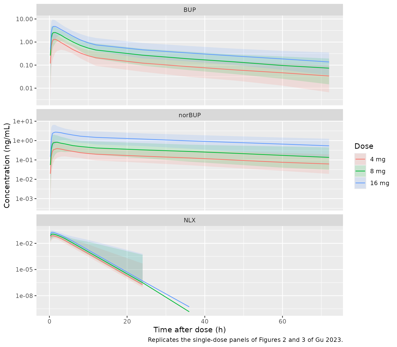
# Replicates the multiple-dose panels of Figures 2 and 3: day 8 of 8 mg QD.
sim_long |>
  dplyr::filter(treatment == "8 mg QD x 8 d", time >= 168) |>
  dplyr::group_by(analyte, time) |>
  dplyr::summarise(
    Q05 = quantile(ipred, 0.05), Q50 = median(ipred), Q95 = quantile(ipred, 0.95),
    .groups = "drop"
  ) |>
  ggplot(aes(time - 168, Q50)) +
  geom_ribbon(aes(ymin = Q05, ymax = Q95), alpha = 0.25) +
  geom_line() +
  facet_wrap(~analyte, scales = "free_y") +
  scale_y_log10() +
  labs(x = "Time after the 8th dose (h)", y = "Concentration (ng/mL)",
       caption = "Replicates the multiple-dose panels of Figures 2 and 3 of Gu 2023.")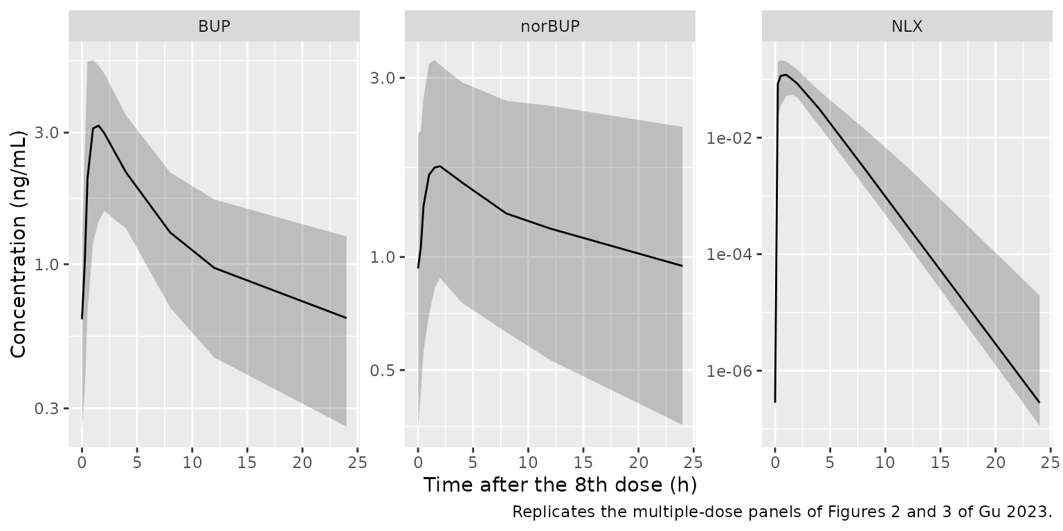
PKNCA validation
The paper’s numerical predictive check (Table S2) reports the median AUC and Cmax of 1000 simulated replicates of each dose group: AUC0-72 h after a single dose, and AUC over the 24 h after the eighth dose in the multiple-dose group. Those medians are the reference here, because they are what the published model itself predicts for these cohorts. Like the paper’s check, the comparison uses simulated observations: residual error is added and values below the assay LLOQ are treated as unquantifiable.
nca_conc <- sim_long |>
  dplyr::filter(!is.na(Cc)) |>
  dplyr::select(id, time, Cc, treatment, analyte)
# Guarantee a pre-dose time-zero record per subject and analyte.
nca_conc <- dplyr::bind_rows(
  nca_conc,
  nca_conc |> dplyr::distinct(id, treatment, analyte) |> dplyr::mutate(time = 0, Cc = 0)
) |>
  dplyr::distinct(id, treatment, analyte, time, .keep_all = TRUE) |>
  dplyr::arrange(analyte, id, time)

nca_dose <- ev_bup |>
  dplyr::filter(evid == 1) |>
  dplyr::select(id, time, amt, treatment)

conc_obj <- PKNCA::PKNCAconc(nca_conc, Cc ~ time | treatment + analyte + id)
dose_obj <- PKNCA::PKNCAdose(nca_dose, amt ~ time | treatment + id)
intervals <- data.frame(
  treatment = arms$treatment,
  start = ifelse(arms$multiple, 168, 0),
  end = ifelse(arms$multiple, 192, 72),
  cmax = TRUE,
  auclast = TRUE
)
nca_res <- PKNCA::pk.nca(PKNCA::PKNCAdata(conc_obj, dose_obj, intervals = intervals))
Comparison against the published predictive check
# Table S2 'NPC result median', converted from ng/L and ng.h/L to ng/mL and
# ng.h/mL. The 8 mg buprenorphine AUC is printed '2768[23264-32262]'; its
# confidence interval shows a dropped digit, so 27680 is used.
published <- tibble::tribble(
  ~analyte, ~treatment, ~auclast, ~cmax,
  "BUP", "4 mg", 13103, 1643,
  "BUP", "8 mg", 27680, 3510,
  "BUP", "16 mg", 45388, 5795,
  "BUP", "8 mg QD x 8 d", 31222, 4108,
  "norBUP", "4 mg", 10949, 479,
  "norBUP", "8 mg", 23826, 1041,
  "norBUP", "16 mg", 77032, 3400,
  "norBUP", "8 mg QD x 8 d", 30246, 2187,
  "NLX", "4 mg", 244, 97,
  "NLX", "8 mg", 379, 147,
  "NLX", "16 mg", 590, 228,
  "NLX", "8 mg QD x 8 d", 420, 142
) |>
  dplyr::mutate(auclast = auclast / 1000, cmax = cmax / 1000)

cmp <- nlmixr2lib::ncaComparisonTable(
  simulated = nca_res,
  reference = published,
  by = c("analyte", "treatment"),
  units = c(cmax = "ng/mL", auclast = "ng*h/mL"),
  tolerance_pct = 20
)
knitr::kable(cmp,
caption = "Simulated median NCA vs. the Table S2 predictive-check medians. * differs by >20%.")| NCA parameter | analyte | treatment | Reference | Simulated | % diff |
|---|---|---|---|---|---|
| Cmax (ng/mL) | BUP | 4 mg | 1.64 | 1.6 | -2.9% |
| Cmax (ng/mL) | BUP | 8 mg | 3.51 | 3.38 | -3.7% |
| Cmax (ng/mL) | BUP | 16 mg | 5.8 | 6.07 | +4.8% |
| Cmax (ng/mL) | BUP | 8 mg QD x 8 d | 4.11 | 3.86 | -6.1% |
| Cmax (ng/mL) | norBUP | 4 mg | 0.479 | 0.49 | +2.2% |
| Cmax (ng/mL) | norBUP | 8 mg | 1.04 | 1.08 | +4.0% |
| Cmax (ng/mL) | norBUP | 16 mg | 3.4 | 3.61 | +6.2% |
| Cmax (ng/mL) | norBUP | 8 mg QD x 8 d | 2.19 | 2.12 | -3.1% |
| Cmax (ng/mL) | NLX | 4 mg | 0.097 | 0.09 | -7.3% |
| Cmax (ng/mL) | NLX | 8 mg | 0.147 | 0.142 | -3.4% |
| Cmax (ng/mL) | NLX | 16 mg | 0.228 | 0.233 | +2.3% |
| Cmax (ng/mL) | NLX | 8 mg QD x 8 d | 0.142 | 0.148 | +4.4% |
| AUClast (ng*h/mL) | BUP | 4 mg | 13.1 | 11.9 | -9.0% |
| AUClast (ng*h/mL) | BUP | 8 mg | 27.7 | 25.9 | -6.6% |
| AUClast (ng*h/mL) | BUP | 16 mg | 45.4 | 46.4 | +2.2% |
| AUClast (ng*h/mL) | BUP | 8 mg QD x 8 d | 31.2 | 29.5 | -5.6% |
| AUClast (ng*h/mL) | norBUP | 4 mg | 10.9 | 10.5 | -3.8% |
| AUClast (ng*h/mL) | norBUP | 8 mg | 23.8 | 23.4 | -1.7% |
| AUClast (ng*h/mL) | norBUP | 16 mg | 77 | 81.2 | +5.4% |
| AUClast (ng*h/mL) | norBUP | 8 mg QD x 8 d | 30.2 | 29.5 | -2.6% |
| AUClast (ng*h/mL) | NLX | 4 mg | 0.244 | 0.228 | -6.7% |
| AUClast (ng*h/mL) | NLX | 8 mg | 0.379 | 0.365 | -3.7% |
| AUClast (ng*h/mL) | NLX | 16 mg | 0.59 | 0.574 | -2.7% |
| AUClast (ng*h/mL) | NLX | 8 mg QD x 8 d | 0.42 | 0.316 | -24.9%* |
pct <- as.numeric(sub("%[*]?$", "", cmp[["% diff"]]))
stopifnot(
  length(pct) == 24L, !anyNA(pct),
  # A mis-transcribed clearance, volume or covariate moves these medians by
  # tens of percent; the medians of 200 subjects sit within a few percent.
  # Realised: median -3%, 90th percentile of |% diff| 7.1%.
  abs(median(pct)) < 10,
  quantile(abs(pct), 0.9) < 20
)
Buprenorphine and norbuprenorphine Cmax and AUC, and the single-dose naloxone values, agree with the published medians to within about 10%. The exception is the naloxone AUC after the eighth dose (about 25% low). In that group 56% of the observed naloxone samples were below the LLOQ (Section 4.1), so the simulated AUC depends heavily on how below-LLOQ values are counted, which the paper does not state for its predictive check; here they count as zero. Without the LLOQ step, the single-dose naloxone AUCs are instead inflated by additive noise in the 72 h tail. The model also reproduces the two dose-dependent features the paper set out to explain: the less than dose-proportional buprenorphine exposure at 16 mg (more swallows, lower bioavailability) and the more than dose-proportional norbuprenorphine exposure at 16 mg (higher Fm).
Dose optimisation (Figures 4-6)
The authors simulated six regimens to steady state and evaluated day 8. The buprenorphine concentration is converted to mu-opioid receptor occupancy with the Emax model of Nasser et al. (2014) quoted in Section 3.5.2 (Emax 91.4%, EC50 0.67 ng/mL). The dosing clock times and the number of swallows used for these simulations are not reported; doses are spaced evenly through the day and every subject swallows twice (the 8 mg median).
regimens <- list(
  "16 mg QD" = list(times = 0, amt = 16),
  "8 mg BID" = list(times = c(0, 12), amt = 8),
  "16 mg + 8 mg" = list(times = c(0, 12), amt = c(16, 8)),
  "8 mg TID" = list(times = c(0, 8, 16), amt = 8),
  "16 mg BID" = list(times = c(0, 12), amt = 16),
  "16 mg + 8 mg + 8 mg" = list(times = c(0, 8, 16), amt = c(16, 8, 8))
)
day8 <- seq(168, 192, by = 0.25)

build_regimen <- function(k, builder) {
  r <- regimens[[k]]
  ids <- (k - 1L) * n_arm + seq_len(n_arm)
  dt <- as.vector(outer(r$times, 24 * 0:7, "+"))
  da <- rep(r$amt, length.out = length(r$times))[rep(seq_along(r$times), 8)]
  ev <- if (identical(builder, "bup")) {
    bup_events(ids, dt, da, c(0, day8), 2)
  } else {
    nlx_events(ids, dt, da, c(0, day8))
  }
  dplyr::mutate(ev, regimen = names(regimens)[k])
}
ev_reg_bup <- dplyr::bind_rows(lapply(seq_along(regimens), build_regimen, builder = "bup"))
ev_reg_nlx <- dplyr::bind_rows(lapply(seq_along(regimens), build_regimen, builder = "nlx"))

rxode2::rxSetSeed(20230120)
reg_bup <- rxode2::rxSolve(mod_bup, events = ev_reg_bup, keep = "regimen") |>
  as.data.frame() |>
  dplyr::filter(time >= 168) |>
  dplyr::mutate(oro = 91.4 * Cc / (0.67 + Cc),
                regimen = factor(regimen, levels = names(regimens)))
reg_nlx <- rxode2::rxSolve(mod_nlx, events = ev_reg_nlx, keep = "regimen") |>
  as.data.frame() |>
  dplyr::filter(time >= 168) |>
  dplyr::mutate(regimen = factor(regimen, levels = names(regimens)))
# Replicates Figure 4: probability of reaching each %T > MSC (3 ng/mL) target
# on day 8.
tmsc <- reg_bup |>
  dplyr::group_by(regimen, id) |>
  dplyr::summarise(pct_t = 100 * mean(Cc >= 3), .groups = "drop")
pta <- tidyr::crossing(target = seq(0, 100, by = 10), tmsc) |>
  dplyr::group_by(regimen, target) |>
  dplyr::summarise(pta = 100 * mean(pct_t >= target), .groups = "drop")
ggplot(pta, aes(target, pta, colour = regimen)) +
  geom_line() + geom_point() +
  labs(x = "%T > MSC target (%)", y = "PTA (%)", colour = "Regimen",
       caption = "Replicates Figure 4 of Gu 2023.")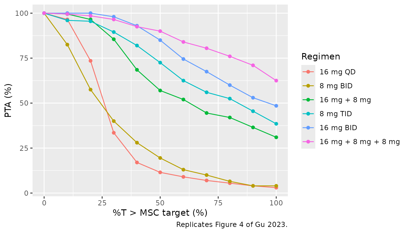
pta |>
  dplyr::filter(target == 50) |>
  dplyr::select(regimen, pta) |>
  dplyr::rename("Regimen" = regimen, "PTA at 50% T > MSC (%)" = pta) |>
knitr::kable(digits = 0)| Regimen | PTA at 50% T > MSC (%) |
|---|---|
| 16 mg QD | 12 |
| 8 mg BID | 20 |
| 16 mg + 8 mg | 57 |
| 8 mg TID | 72 |
| 16 mg BID | 85 |
| 16 mg + 8 mg + 8 mg | 90 |
For 8 mg TID the simulated probability of keeping buprenorphine above 3 ng/mL for at least half of day 8 is close to the paper’s ~70%. The two 16 mg BID and 16 + 8 + 8 mg regimens come out higher than the paper’s ~70%, as expected from giving every 16 mg dose the two-swallow bioavailability; the 16 mg group in the trial swallowed a median 6.5 times.
# Replicates Figure 5: receptor occupancy on day 8, median and 90% PI.
oro_sum <- reg_bup |>
  dplyr::group_by(regimen, time) |>
  dplyr::summarise(Q05 = quantile(oro, 0.05), Q50 = median(oro),
                   Q95 = quantile(oro, 0.95), .groups = "drop")
ggplot(oro_sum, aes(time - 168, Q50)) +
  geom_ribbon(aes(ymin = Q05, ymax = Q95), alpha = 0.25) +
  geom_line() +
  geom_hline(yintercept = 70, linetype = "dashed") +
  facet_wrap(~regimen) +
  labs(x = "Time on day 8 (h)", y = "mu-opioid receptor occupancy (%)",
       caption = "Replicates Figure 5 of Gu 2023.")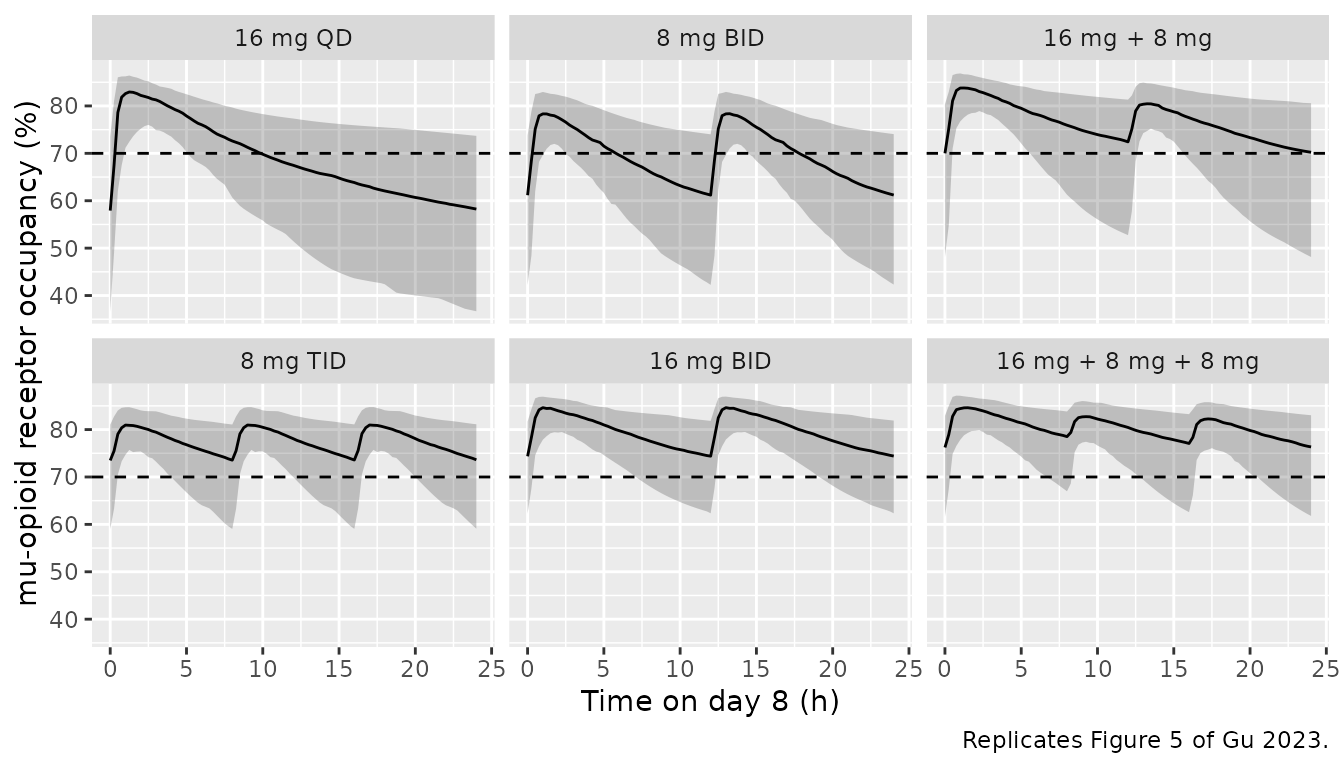
# Replicates Figure 6: naloxone concentration on day 8, median and 90% PI,
# against the 4.6 ng/mL withdrawal threshold.
nlx_sum <- reg_nlx |>
  dplyr::group_by(regimen, time) |>
  dplyr::summarise(Q05 = quantile(Cc, 0.05), Q50 = median(Cc),
                   Q95 = quantile(Cc, 0.95), .groups = "drop")
ggplot(nlx_sum, aes(time - 168, Q50, colour = regimen, fill = regimen)) +
  geom_ribbon(aes(ymin = Q05, ymax = Q95), alpha = 0.15, colour = NA) +
  geom_line() +
  geom_hline(yintercept = 4.6, linetype = "dashed", colour = "red") +
  scale_y_log10() +
  labs(x = "Time on day 8 (h)", y = "Naloxone (ng/mL)",
       colour = "Regimen", fill = "Regimen",
       caption = "Replicates Figure 6 of Gu 2023.")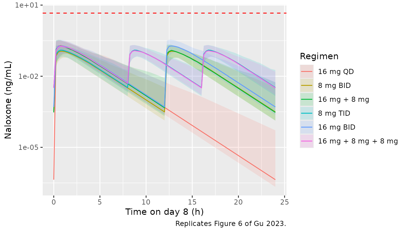
nlx_cmax_tid <- reg_nlx |>
  dplyr::filter(regimen == "8 mg TID") |>
  dplyr::group_by(id) |>
  dplyr::summarise(cmax = max(Cc), .groups = "drop")
oro_tid <- oro_sum |> dplyr::filter(regimen == "8 mg TID")
stopifnot(
  # Section 4.5: with 8 mg TID the naloxone peak stays below 4.6 ng/mL in
  # more than 95% of patients (the simulated 95th percentile is far below).
  quantile(nlx_cmax_tid$cmax, 0.95) < 4.6,
  # Section 4.5: 8 mg TID achieves and maintains occupancy of at least 70%
  # (median over day 8). Realised minimum 73.5%; the standard error of a
  # 200-subject median occupancy is under 1 percentage point.
  min(oro_tid$Q50) > 70
)
Assumptions and deviations
-
Norbuprenorphine CL and Vc. Table 4 prints 22.2
against ‘CL norBUP /Fm, L/h’ and 264 against ‘V C norBUP /Fm, L’, with
the matching IIV rows (119.6% and 50.5%). The control stream assigns
them the other way round (
TVV4=THETA(9)with initial value 22.2,TVCLM=THETA(10)with 264;$OMEGA1.43 on V4 and 0.255 on CLM). The control-stream reading is used: it reproduces the Table S2 norbuprenorphine medians (table above), whereas a clearance of 22.2 L/h would raise norbuprenorphine AUC about 12-fold. -
Centring of the number of swallows. The control
stream centres on 3 swallows (
NOS-3), not on the Table 1 median of 2 that the general covariate equation of Section 3.3 would imply; the stream is used. -
Transit absorption as an explicit chain. The
control stream writes the Savic transit input in closed form
(
DADT(1)), driven by the time since the dose, and removes the dose record’s amount from the depot withF1 = 0. With the number of transit compartments fixed at the integer 8, a chain of 9 compartments sharing the rate constantktr = 9 / MTTdelivers exactly the same input, and the dose is given to its first compartment. The chain is used because the closed-form input is zero at the dose and lasts only about 0.2 h, so an ODE solver stepping between sparse observation times can pass over it entirely. Two consequences: the dose is entered ontransit1, and a dose given while an earlier one is still in transit is superposed rather than restarting the input; with a mean transit time of 0.23 h this has no effect at any practical dosing interval. -
Stirling factor in the transit input. The control
stream normalises the input with Stirling’s approximation to log(n!), so
at n = 8 it absorbs 1.0105 times the bioavailable dose. The factor is
reproduced on
f(transit1), and the mass-balance check above carries it explicitly. -
Transit input driven by
amt. The control stream reads the dose for the transit input from itsDOSEdata column; the model uses the dose record’samt, soamtandDOSE_BPN_SL_MGcarry the same value. -
Naloxone dose units. The naloxone model’s
bioavailability is a fixed 0.01 at the 8 mg level (Table 3, citing
McDonald et al. 2018), and the dose record carries the labelled
buprenorphine strength, not the naloxone content: with
amt = 8the model reproduces the Table S2 naloxone medians and the Discussion’s dose-normalised AUC (39 ng.h/L per mg at 8 mg), whereas entering the 2 mg of naloxone would give exposures 4-fold too low. The maintainers kept the published parameterisation rather than re-expressing it per mg of naloxone with F = 0.04. - Units. Doses are tablet labels (2 mg buprenorphine hydrochloride + 0.5 mg naloxone hydrochloride per tablet, Section 2.1); no salt correction is applied, as in the source. Norbuprenorphine is carried in buprenorphine-mass units (no molecular-weight conversion in the control stream).
-
Inter-individual variability. Tables 3 and 4 print
IIV as
sqrt(omega^2) * 100; for example 135.6% for buprenorphine Vc is the square root of the control-stream estimate 1.84. Variances are therefore(CV/100)^2. -
Naloxone structure. Table S3 describes the final
naloxone model as “two-compartment”, but the main text (Sections 4.4 and
5) and the control stream (
ADVAN2 TRANS2) use one compartment, which is what is packaged. -
Covariates screened but not retained (age, weight,
disease state for both drugs; number of swallows for naloxone) are
listed in
covariatesDataExcluded. - Simulation design for Figures 4-6. Dosing clock times and the swallow counts behind the paper’s “NOS-adjusted” doses are not reported; doses are spaced evenly and every virtual subject swallows twice. The PTA values above are therefore indicative only: the paper reports PTA near 70% at the 50% target for 8 mg TID, 16 mg BID and 16 + 8 + 8 mg. For norbuprenorphine, a 16 mg dose in a mixed regimen switches Fm only while it is the most recent dose; this does not affect buprenorphine or the figures above.
- No erratum or correction notice for this article was found as of 2026-10-15.