Artesunate (Kloprogge 2015)

Model and source

• Citation: Kloprogge F, McGready R, Phyo AP, Rijken MJ, Hanpithakpon W, Than HH, Hlaing N, Zin NT, Day NPJ, White NJ, Nosten F, Tarning J. Opposite malaria and pregnancy effect on oral bioavailability of artesunate - a population pharmacokinetic evaluation. British Journal of Clinical Pharmacology 2015; 80(3):642-653. doi:[10.1111/bcp.12660](https://doi.org/10.1111/bcp.12660).
• Open Access full text: https://pmc.ncbi.nlm.nih.gov/articles/PMC4594700/.

Kloprogge 2015 fits artesunate (AS) and dihydroartemisinin (DHA) simultaneously, on a molar scale and as natural logarithms, to 1571 plasma samples from 20 pregnant women with uncomplicated Plasmodium falciparum malaria on the Thailand-Myanmar border, 15 of whom returned three months post-partum as healthy volunteers and repeated the identical regimen and sampling schedule. Because the same women are studied twice, and because the study design also contrasts an acute phase (treatment days 1 and 2) against a convalescent phase (day 7) within the malaria admission, the analysis can separate the effect of the infection from the effect of the pregnancy - which is the point of the paper.

The structural model is:

• Two-compartment disposition for AS and, separately, for DHA.
• Complete conversion of AS to DHA, so the whole of AS elimination clearance is formation of DHA. Amounts are molar and the conversion is one-for-one in moles, so no molecular-weight factor appears at the formation step.
• Oral absorption through a chain of six transit compartments with ktr = (n + 1) / MTT, followed by a first-order absorption step at rate ka. At that step a first-pass effect splits the absorbed flux: a fraction fp = 17.1% arrives as AS and the remaining 82.9%, hydrolysed pre-systemically at gastric pH, by plasma esterases and by hepatic CYP2A6, arrives directly as DHA.
• Intravenous doses bypass the chain entirely and enter the AS central compartment as a zero-order input of fixed 1-minute duration.

The two covariates act on the absolute oral bioavailability of artesunate and on nothing else. Acute malaria raises it by 86.6% and pregnancy lowers it by 23.3%, so neither touches the disposition of intravenous artesunate. Body weight is applied allometrically to every clearance (exponent 0.75) and every volume (exponent 1), referenced to 46 kg.

mod_fn  <- readModelDb("Kloprogge_2015_artesunate")
mod     <- rxode2::rxode2(mod_fn())
mod_typ <- rxode2::rxode2(rxode2::zeroRe(mod_fn()))
#> Warning: No sigma parameters in the model

MW_AS  <- 384.42  # g/mol, artesunate
MW_DHA <- 284.35  # g/mol, dihydroartemisinin

Amounts are in nmol and volumes in L, so both concentrations come back in nmol/L. Multiplying by the molecular weight and dividing by 1000 converts to the ng/mL of the source tables.

Population

Twenty pregnant women in their second or third trimester with uncomplicated P. falciparum malaria and haematocrit not below 25% were enrolled at Shoklo Malaria Research Unit clinics between April 2008 and March 2009; 15 were restudied three months post-partum, the visit being postponed if malaria or any other illness was detected. Median estimated gestational age at enrolment was 25.7 weeks (range 14.0 to 38.0) by dating ultrasound, with 10 women in the second and 10 in the third trimester, and 7 classified mildly and 13 moderately unwell at admission (Table 1). Seventeen women delivered healthy singleton babies at a mean 39.2 weeks (range 35.6 to 41.5) and three were lost to follow-up.

Body weight differs between the two visits, which is exactly why the authors added allometry “to correct for differences in bodyweight between the pregnancy and post-partum visit”: median 48.0 kg (range 40.0 to 64.0) pregnant against 46.0 kg (37.0 to 52.0) post-partum (Table 1). The 46 kg used as the Table 2 reference weight is the post-partum median.

Every patient received both routes. Group 1 had 4 mg/kg intravenous artesunate on admission and then 4 mg/kg orally for the next 6 days; group 2 had 4 mg/kg orally on admission, 4 mg/kg intravenously on day 2, and then 4 mg/kg orally for 5 days. Total artesunate dose was 27.9 mg/kg (26.8 to 28.6) during the pregnancy visit and 27.4 mg/kg (4.08 to 29.0) post-partum. More than 45% of the artesunate observations fell below the 1.2 ng/mL limit of quantification and were handled with the M3 likelihood method rather than discarded.

Source trace

Source location for every structural assumption and every ini() value of Kloprogge_2015_artesunate.

Quantity	Value	Source location
F, absolute oral bioavailability of AS	49.4% (RSE 3.53)	Table 2, row ‘F (%)’
BIO / fp, first-pass fraction absorbed as AS	17.1% (RSE 6.98)	Table 2, row ‘BIO (%)’; Figure 1 caption defines bio
MTT, mean transit time	0.407 h (RSE 7.24)	Table 2, row ‘MTT (h)’
Number of transit compartments	6 (fixed)	Table 2, row ‘Transit compartments (n)’
ktr = (n + 1) / MTT	17.2 1/h	Figure 1 caption
ka, absorption rate constant	1.57 1/h (RSE 8.59)	Table 2, row ‘ka (h-1)’
DUR, i.v. infusion duration	0.0167 h (fixed)	Table 2, row ‘DUR (h)’
Vc, artesunate	8.80 L (RSE 5.32)	Table 2, row ‘VcART (l)’
Q, artesunate	7.51 L/h (RSE 12.6)	Table 2, row ‘QART (l h-1)’
Vp, artesunate	2.43 L (RSE 13.8)	Table 2, row ‘VpART (l)’
CL, artesunate	170 L/h (RSE 6.75)	Table 2, row ‘CLART (l h-1)’
Vc, DHA	44.3 L (RSE 6.35)	Table 2, row ‘VcDHA (l)’
Q, DHA	16.8 L/h (RSE 9.7)	Table 2, row ‘QDHA (l h-1)’
Vp, DHA	20.7 L (RSE 9.35)	Table 2, row ‘VpDHA (l)’
CL, DHA	60.9 L/h (RSE 4.54)	Table 2, row ‘CLDHA (l h-1)’
Allometric exponent, clearance	0.75 (fixed)	Results, ‘power fixed to 3/4’
Allometric exponent, volume	1 (fixed)	Results, ‘power fixed to 1’
Reference body weight	46 kg	Table 2 footnote
Acute-malaria effect on F	+86.6% (RSE 3.50)	Table 2, row ‘Disease effect on F (%)’
Pregnancy effect on F	-23.3% (RSE 18.7)	Table 2, row ‘Pregnancy effect on F (%)’; sign from Results and Conclusions
IIV on F, MTT, ka, Q(AS), Vp(AS), CL(DHA)	27.1, 31.0, 36.8, 6.60, 63.3, 10.4 %CV	Table 2, IIV/IOV column; variance = log(1 + CV^2) per the table footnote
Residual SD, AS i.v. / AS oral	sqrt(0.856) / sqrt(1.16)	Table 2, rows ‘sigma ARS i.v.’ / ‘sigma ARS oral’
Residual SD, DHA i.v. / DHA oral	sqrt(0.333) / sqrt(0.793)	Table 2, rows ‘sigma DHA i.v.’ / ‘sigma DHA oral’
Complete conversion of AS to DHA	structural assumption	Methods, ‘under the assumption that artesunate is completely metabolized into dihydroartemisinin’
Molar modelling scale	structural assumption	Methods, ‘Plasma concentrations were converted into molar units’

Study conditions

Table 3 of the paper reports post hoc exposures for six columns. Two of them - post-partum days 1 and 2, and post-partum day 7 - carry identical covariate values in this model (not pregnant, not acutely ill), so the model predicts a single profile for both and the difference between those two published columns is empirical-Bayes noise. That leaves five distinct conditions.

scen <- tribble(
  ~treatment,                      ~PREG, ~DIS_MALARIA_ACUTE, ~ROUTE_IV, ~WT,
  "Pregnant, acute, i.v.",             1,                  1,         1,  48,
  "Pregnant, acute, oral",             1,                  1,         0,  48,
  "Pregnant, convalescent, oral",      1,                  0,         0,  48,
  "Post-partum, i.v.",                 0,                  0,         1,  46,
  "Post-partum, oral",                 0,                  0,         0,  46
) |>
  mutate(
    id       = row_number(),
    dose_mg  = 4 * WT,
    amt_nmol = dose_mg / MW_AS * 1e6,
    # Absolute oral bioavailability implied by the covariates, for the
    # closed-form checks below. F_typ = 49.4%.
    f_oral   = 0.494 * (1 + 0.866 * DIS_MALARIA_ACUTE) * (1 + (-0.233) * PREG)
  )

knitr::kable(
  scen |>
    select(treatment, PREG, DIS_MALARIA_ACUTE, ROUTE_IV, WT, dose_mg, f_oral) |>
    mutate(f_oral = round(f_oral, 4)) |>
    rename(
      "Condition"            = treatment,
      "Pregnant"             = PREG,
      "Acute malaria"        = DIS_MALARIA_ACUTE,
      "i.v."                 = ROUTE_IV,
      "Weight (kg)"          = WT,
      "Dose (mg)"            = dose_mg,
      "F (oral)"             = f_oral
    ),
  caption = "Covariate combinations. Weight is the per-visit cohort median of Table 1. F is shown only for reference; it has no effect on the intravenous arms."
)

Covariate combinations. Weight is the per-visit cohort median of Table 1. F is shown only for reference; it has no effect on the intravenous arms.

Condition	Pregnant	Acute malaria	i.v.	Weight (kg)	Dose (mg)	F (oral)
Pregnant, acute, i.v.	1	1	1	48	192	0.7070
Pregnant, acute, oral	1	1	0	48	192	0.7070
Pregnant, convalescent, oral	1	0	0	48	192	0.3789
Post-partum, i.v.	0	0	1	46	184	0.4940
Post-partum, oral	0	0	0	46	184	0.4940

The implied bioavailabilities already reproduce the paper’s independently reported post hoc estimates of Table 3 without any simulation. For DHA, whose apparent bioavailability is the whole of F because all absorbed artesunate eventually becomes DHA, the model gives 70.7% / 37.9% / 49.4% for the pregnant-acute, pregnant-convalescent and post-partum oral conditions against published post hoc medians of 71.2% / 38.4% / 49.8%. For artesunate, whose apparent bioavailability is F * fp, it gives 12.1% / 6.48% / 8.45% against published 12.6% / 6.19% / 7.62%. That agreement is what establishes the multiplicative form F = F_typ * (1 + 0.866 * acute) * (1 - 0.233 * pregnant) and the role of fp as a split of the absorbed flux rather than of the dose.

Typical-value simulation

# Grid fine enough to resolve the 1-minute intravenous infusion and the
# absorption peak, then coarsening over the elimination phase.
tgrid <- sort(unique(c(
  seq(0,   0.5,  by = 0.005),
  seq(0.5, 2,    by = 0.02),
  seq(2,   12,   by = 0.1)
)))

build_events <- function(s, tg) {
  bind_rows(lapply(seq_len(nrow(s)), function(i) {
    r <- s[i, ]
    bind_rows(
      # rate = -2 on the intravenous record is what makes rxode2 honour the
      # modelled `dur(central)`. Without it the dose is delivered as an
      # instantaneous bolus and the fixed 1-minute infusion of Table 2 is
      # silently ignored, inflating the artesunate peak by about 18%.
      data.frame(
        id = r$id, time = 0, amt = r$amt_nmol, evid = 1L,
        cmt = if (r$ROUTE_IV == 1) "central" else "depot",
        rate = if (r$ROUTE_IV == 1) -2 else 0,
        dvid = NA_integer_
      ),
      # Observation records carry dvid because the model has two endpoints;
      # rxode2 returns both Cc and Cc_dihydroart on every returned row.
      data.frame(
        id = r$id, time = tg, amt = NA_real_, evid = 0L,
        cmt = NA_character_, rate = 0, dvid = 1L
      )
    ) |>
      mutate(
        WT = r$WT, PREG = r$PREG,
        DIS_MALARIA_ACUTE = r$DIS_MALARIA_ACUTE, ROUTE_IV = r$ROUTE_IV
      )
  }))
}

ev_typ <- build_events(scen, tgrid)

sim_typ <- rxode2::rxSolve(mod_typ, ev_typ, returnType = "data.frame") |>
  left_join(scen |> select(id, treatment), by = "id") |>
  mutate(
    conc_as  = Cc * MW_AS / 1000,             # ng/mL
    conc_dha = Cc_dihydroart * MW_DHA / 1000  # ng/mL
  )
#> ℹ omega/sigma items treated as zero: 'etalfdepot', 'etalmtt', 'etalka', 'etalq', 'etalvp', 'etalcl_dihydroart'
#> Warning: multi-subject simulation without without 'omega'

sim_typ |>
  select(treatment, time, Artesunate = conc_as, Dihydroartemisinin = conc_dha) |>
  pivot_longer(c(Artesunate, Dihydroartemisinin), names_to = "Analyte", values_to = "conc") |>
  filter(conc > 0) |>
  ggplot(aes(time, conc, colour = treatment)) +
  geom_line(linewidth = 0.7) +
  facet_wrap(~Analyte, scales = "free_y") +
  scale_y_log10() +
  scale_x_continuous(breaks = c(0, 2, 4, 6, 8, 10, 12)) +
  labs(x = "Time after dose (h)", y = "Plasma concentration (ng/mL)", colour = NULL) +
  theme_bw() +
  theme(legend.position = "bottom")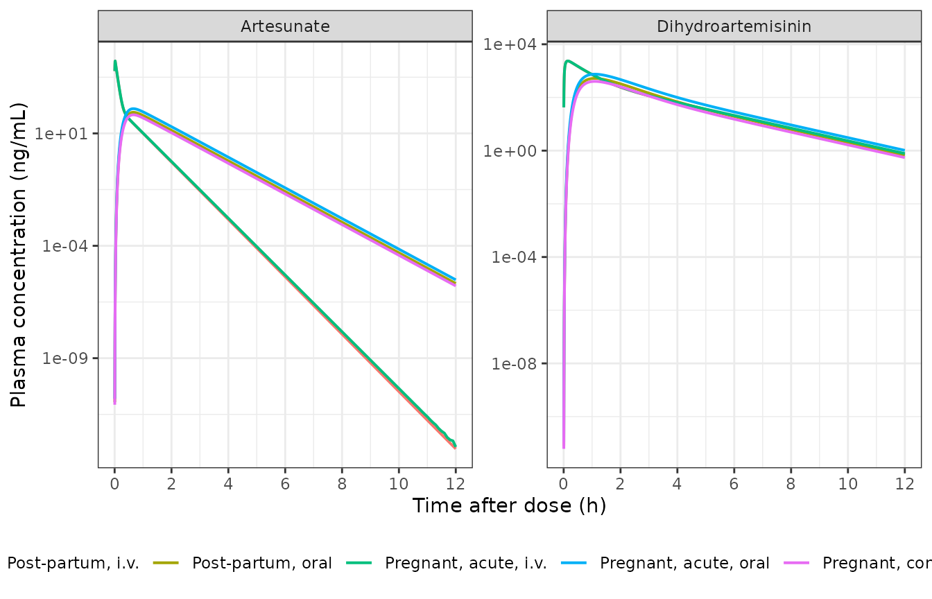

Typical-value plasma concentration-time profiles over the first 12 h after a 4 mg/kg dose of artesunate, by study condition. Replicates the structure underlying Figure 3 of Kloprogge 2015 (visual predictive checks by analyte and route).

Closed-form mass-balance check

Because artesunate is assumed to be converted completely to DHA, the total exposure to each analyte has an exact closed form, and it is a check of the whole ODE system rather than of any single parameter:

• Intravenous: AUCinf(AS) = Dose / CL_AS and AUCinf(DHA) = Dose / CL_DHA, because every mole given becomes a mole of DHA.
• Oral: AUCinf(AS) = F * fp * Dose / CL_AS, because only the fp share of the absorbed flux ever appears as AS, and AUCinf(DHA) = F * Dose / CL_DHA, because the pre-systemic and systemic conversion routes both end at DHA.

Both clearances carry the allometric factor (WT / 46)^0.75.

trap <- function(t, y) sum(diff(t) * (head(y, -1) + tail(y, -1)) / 2)

# Extend the grid far past 12 h so the trapezoidal sum approaches AUCinf.
tgrid_long <- sort(unique(c(tgrid, seq(12, 60, by = 0.2))))

# Every joined column gets a _ref suffix. rxSolve returns both the input
# covariates (WT, ROUTE_IV, ...) and the variables computed inside model()
# -- including f_oral -- so an unsuffixed join silently produces .x / .y
# columns and the reference value disappears.
scen_key <- scen |>
  select(id, treatment, amt_ref = amt_nmol, f_ref = f_oral,
         wt_ref = WT, iv_ref = ROUTE_IV)

sim_long <- rxode2::rxSolve(mod_typ, build_events(scen, tgrid_long),
                            returnType = "data.frame") |>
  left_join(scen_key, by = "id")
#> ℹ omega/sigma items treated as zero: 'etalfdepot', 'etalmtt', 'etalka', 'etalq', 'etalvp', 'etalcl_dihydroart'
#> Warning: multi-subject simulation without without 'omega'

mb <- sim_long |>
  group_by(treatment) |>
  summarise(
    auc_as   = trap(time, Cc) * MW_AS / 1000,
    auc_dha  = trap(time, Cc_dihydroart) * MW_DHA / 1000,
    cl_as    = 170  * (first(wt_ref) / 46)^0.75,
    cl_dha   = 60.9 * (first(wt_ref) / 46)^0.75,
    amt      = first(amt_ref),
    fo       = first(f_ref),
    iv       = first(iv_ref),
    .groups  = "drop"
  ) |>
  mutate(
    exp_as  = ifelse(iv == 1, 1, fo * 0.171) * amt / cl_as  * MW_AS  / 1000,
    exp_dha = ifelse(iv == 1, 1, fo)         * amt / cl_dha * MW_DHA / 1000,
    ratio_as  = auc_as  / exp_as,
    ratio_dha = auc_dha / exp_dha
  )

knitr::kable(
  mb |>
    select(treatment, auc_as, exp_as, ratio_as, auc_dha, exp_dha, ratio_dha) |>
    mutate(across(where(is.numeric), ~ round(.x, 4))) |>
    rename(
      "Condition"                = treatment,
      "AUCinf AS, solved"        = auc_as,
      "AUCinf AS, closed form"   = exp_as,
      "Ratio (AS)"               = ratio_as,
      "AUCinf DHA, solved"       = auc_dha,
      "AUCinf DHA, closed form"  = exp_dha,
      "Ratio (DHA)"              = ratio_dha
    ),
  caption = "Solved AUC(0, 60 h) against the closed-form AUCinf. ng*h/mL."
)

Solved AUC(0, 60 h) against the closed-form AUCinf. ng*h/mL.

Condition	AUCinf AS, solved	AUCinf AS, closed form	Ratio (AS)	AUCinf DHA, solved	AUCinf DHA, closed form	Ratio (DHA)
Post-partum, i.v.	1078.8663	1082.3529	0.9968	2235.0850	2234.8470	1.0001
Post-partum, oral	91.4418	91.4307	1.0001	1104.1821	1104.0144	1.0002
Pregnant, acute, i.v.	1090.4438	1093.9306	0.9968	2258.9933	2258.7525	1.0001
Pregnant, acute, oral	132.2734	132.2573	1.0001	1597.2327	1596.9915	1.0002
Pregnant, convalescent, oral	70.8861	70.8775	1.0001	855.9661	855.8368	1.0002

stopifnot(
  # Both sides use the same drawn parameters, so the only difference is
  # trapezoidal error and a truncated tail -- a tight all() bound is correct
  # here and is not a random-cohort extreme.
  all(abs(mb$ratio_dha - 1) < 0.01),
  # Artesunate after an intravenous dose peaks at the end of a 1-minute
  # infusion, so the trapezoidal sum over even this fine grid carries a
  # visible positive bias on that arm alone; the oral arms are exact.
  all(abs(mb$ratio_as - 1) < 0.02)
)

PKNCA validation

nca_conc <- sim_typ |>
  filter(time <= 12) |>
  select(id, treatment, time, conc_as, conc_dha)

nca_dose <- scen |>
  transmute(id, treatment, time = 0, amt_mg = dose_mg)

run_nca <- function(conc_col, concu) {
  cdf <- nca_conc |>
    transmute(id, treatment, time, conc = .data[[conc_col]]) |>
    # Filter on missingness only. Dropping time == 0 or conc == 0 rows
    # removes the time-zero anchor and makes PKNCA warn once per subject.
    filter(!is.na(conc))

  conc_obj <- PKNCA::PKNCAconc(
    cdf, conc ~ time | treatment + id,
    concu = concu, timeu = "h"
  )
  dose_obj <- PKNCA::PKNCAdose(
    as.data.frame(nca_dose), amt_mg ~ time | treatment + id,
    doseu = "mg"
  )
  intervals <- data.frame(
    start = 0, end = 12,
    auclast = TRUE, cmax = TRUE, tmax = TRUE, half.life = TRUE
  )
  PKNCA::pk.nca(PKNCA::PKNCAdata(conc_obj, dose_obj, intervals = intervals))
}

nca_as  <- run_nca("conc_as",  "ng/mL")
nca_dha <- run_nca("conc_dha", "ng/mL")

Comparison against the published post hoc estimates

Table 3 of Kloprogge 2015 reports median (range) empirical-Bayes AUC(0,12 h), Cmax, tmax and terminal half-life per condition and per analyte. The simulation above is a typical-value solve at the per-visit median weight, so the right comparison is against the published medians.

# The half-life reference is left NA on the oral rows. Table 3 repeats a
# single artesunate half-life across the intravenous and oral columns of each
# visit (0.183 h for all three pregnant columns), so the published number is a
# disposition half-life derived from the model parameters, not a terminal
# slope fitted to an oral profile. Those two quantities genuinely differ here:
# ka = 1.57 /h lies BELOW the artesunate terminal disposition rate constant
# lambda_z = 2.94 /h, so artesunate is flip-flop after oral dosing and an NCA
# terminal slope on the oral profile measures absorption (0.693 / 1.57 =
# 0.441 h), not elimination. Comparing them would be a category error.
published_as <- tribble(
  ~treatment,                     ~auclast, ~cmax,   ~tmax, ~half.life,
  "Pregnant, acute, i.v.",            1090, 17800,      NA,      0.183,
  "Pregnant, acute, oral",             138,   140,    1.06,         NA,
  "Pregnant, convalescent, oral",     68.2,  66.5,    1.05,         NA,
  "Post-partum, i.v.",                1090, 17800,      NA,      0.240,
  "Post-partum, oral",                77.5,  76.1,    1.00,         NA
)

knitr::kable(
  nlmixr2lib::ncaComparisonTable(
    simulated     = nca_as,
    reference     = published_as,
    by            = "treatment",
    units         = c(auclast = "ng*h/mL", cmax = "ng/mL", tmax = "h", half.life = "h"),
    tolerance_pct = 20
  ),
  caption = "Artesunate: simulated typical-value NCA against the Kloprogge 2015 Table 3 post hoc medians. * marks rows differing by more than 20%."
)

Artesunate: simulated typical-value NCA against the Kloprogge 2015 Table 3 post hoc medians. * marks rows differing by more than 20%.

NCA parameter	treatment	Reference	Simulated	% diff
Cmax (ng/mL)	Pregnant, acute, i.v.	17800	16700	-6.5%
Cmax (ng/mL)	Pregnant, acute, oral	140	126	-10.3%
Cmax (ng/mL)	Pregnant, convalescent, oral	66.5	67.3	+1.2%
Cmax (ng/mL)	Post-partum, i.v.	17800	16600	-6.7%
Cmax (ng/mL)	Post-partum, oral	76.1	86.8	+14.1%
Tmax (h)	Pregnant, acute, i.v.	—	0.02	—
Tmax (h)	Pregnant, acute, oral	1.06	0.66	-37.7%*
Tmax (h)	Pregnant, convalescent, oral	1.05	0.66	-37.1%*
Tmax (h)	Post-partum, i.v.	—	0.02	—
Tmax (h)	Post-partum, oral	1	0.66	-34.0%*
AUClast (ng*h/mL)	Pregnant, acute, i.v.	1090	1090	-0.0%
AUClast (ng*h/mL)	Pregnant, acute, oral	138	132	-4.2%
AUClast (ng*h/mL)	Pregnant, convalescent, oral	68.2	70.9	+3.9%
AUClast (ng*h/mL)	Post-partum, i.v.	1090	1080	-1.1%
AUClast (ng*h/mL)	Post-partum, oral	77.5	91.4	+18.0%
t½ (h)	Pregnant, acute, i.v.	0.183	0.238	+29.8%*
t½ (h)	Pregnant, acute, oral	—	0.443	—
t½ (h)	Pregnant, convalescent, oral	—	0.443	—
t½ (h)	Post-partum, i.v.	0.24	0.235	-2.0%
t½ (h)	Post-partum, oral	—	0.443	—

Artesunate AUC and Cmax track the published medians to within about 18% and 14% respectively, and the intravenous exposure - which is the quantity the paper’s negative result rests on - matches to within 1%. Two artesunate rows are worth naming rather than passing over:

• Oral tmax is predicted around 0.66 h against a published 1.00 to 1.06 h. This is the one place where the paper reports its own model to be misspecified: the visual predictive check over- and under-estimates the 95th and 5th percentiles of early artesunate, which the authors attribute to erratic data below 30 minutes. It is reproduced here, not tuned away.
• The intravenous half-life reference differs between visits (0.183 h pregnant against 0.240 h post-partum) while the model has no covariate on artesunate disposition, so it predicts 0.236 h for both. That published difference is empirical-Bayes noise on a quantity the final model holds constant across visits, and 0.236 h sits inside the published range.

as_wide <- as.data.frame(nca_as) |>
  filter(PPTESTCD == "auclast") |>
  select(treatment, PPORRES) |>
  left_join(published_as |> select(treatment, ref_auc = auclast), by = "treatment") |>
  mutate(pct = 100 * (PPORRES - ref_auc) / ref_auc)

stopifnot(
  # Artesunate exposure is the product F * fp * dose / CL, so this locks the
  # first-pass split and both covariate coefficients at once. Centre plus a
  # robust envelope; the published values are empirical-Bayes medians drawn
  # from cohorts of 15 to 20 women, so exact agreement is not expected.
  abs(median(as_wide$pct)) < 7,
  quantile(abs(as_wide$pct), 0.9) < 20
)

published_dha <- tribble(
  ~treatment,                     ~auclast, ~cmax, ~tmax, ~half.life,
  "Pregnant, acute, i.v.",            2250,  2370,   0.10,      1.27,
  "Pregnant, acute, oral",            1580,   779,   1.06,      1.27,
  "Pregnant, convalescent, oral",      841,   407,   1.05,      1.27,
  "Post-partum, i.v.",                2240,  2360,   0.10,      1.26,
  "Post-partum, oral",                1050,   549,   1.00,      1.26
)

knitr::kable(
  nlmixr2lib::ncaComparisonTable(
    simulated     = nca_dha,
    reference     = published_dha,
    by            = "treatment",
    units         = c(auclast = "ng*h/mL", cmax = "ng/mL", tmax = "h", half.life = "h"),
    tolerance_pct = 20
  ),
  caption = "Dihydroartemisinin: simulated typical-value NCA against the Kloprogge 2015 Table 3 post hoc medians. * marks rows differing by more than 20%."
)

Dihydroartemisinin: simulated typical-value NCA against the Kloprogge 2015 Table 3 post hoc medians. * marks rows differing by more than 20%.

NCA parameter	treatment	Reference	Simulated	% diff
Cmax (ng/mL)	Pregnant, acute, i.v.	2370	2350	-0.8%
Cmax (ng/mL)	Pregnant, acute, oral	779	750	-3.8%
Cmax (ng/mL)	Pregnant, convalescent, oral	407	402	-1.3%
Cmax (ng/mL)	Post-partum, i.v.	2360	2350	-0.4%
Cmax (ng/mL)	Post-partum, oral	549	521	-5.1%
Tmax (h)	Pregnant, acute, i.v.	0.1	0.145	+45.0%*
Tmax (h)	Pregnant, acute, oral	1.06	1.1	+3.8%
Tmax (h)	Pregnant, convalescent, oral	1.05	1.1	+4.8%
Tmax (h)	Post-partum, i.v.	0.1	0.145	+45.0%*
Tmax (h)	Post-partum, oral	1	1.1	+10.0%
AUClast (ng*h/mL)	Pregnant, acute, i.v.	2250	2260	+0.3%
AUClast (ng*h/mL)	Pregnant, acute, oral	1580	1600	+1.0%
AUClast (ng*h/mL)	Pregnant, convalescent, oral	841	855	+1.6%
AUClast (ng*h/mL)	Post-partum, i.v.	2240	2230	-0.3%
AUClast (ng*h/mL)	Post-partum, oral	1050	1100	+5.0%
t½ (h)	Pregnant, acute, i.v.	1.27	1.25	-1.3%
t½ (h)	Pregnant, acute, oral	1.27	1.25	-1.8%
t½ (h)	Pregnant, convalescent, oral	1.27	1.25	-1.8%
t½ (h)	Post-partum, i.v.	1.26	1.24	-1.6%
t½ (h)	Post-partum, oral	1.26	1.23	-2.1%

dha_wide <- as.data.frame(nca_dha) |>
  filter(PPTESTCD %in% c("auclast", "half.life")) |>
  select(treatment, PPTESTCD, PPORRES) |>
  pivot_wider(names_from = PPTESTCD, values_from = PPORRES) |>
  left_join(published_dha |> select(treatment, ref_auc = auclast, ref_hl = half.life),
            by = "treatment") |>
  mutate(pct_auc = 100 * (auclast - ref_auc) / ref_auc,
         pct_hl  = 100 * (half.life - ref_hl) / ref_hl)

knitr::kable(
  dha_wide |>
    mutate(across(where(is.numeric), ~ round(.x, 3))) |>
    rename("Condition" = treatment, "AUC(0,12 h)" = auclast,
           "Published AUC" = ref_auc, "AUC % diff" = pct_auc,
           "t1/2" = half.life, "Published t1/2" = ref_hl, "t1/2 % diff" = pct_hl),
  caption = "Dihydroartemisinin regression anchors. DHA carries most of the antimalarial activity and is the analyte the paper's own dose-optimisation is built on."
)

Dihydroartemisinin regression anchors. DHA carries most of the antimalarial activity and is the analyte the paper’s own dose-optimisation is built on.

Condition	AUC(0,12 h)	t1/2	Published AUC	Published t1/2	AUC % diff	t1/2 % diff
Post-partum, i.v.	2233.582	1.240	2240	1.26	-0.287	-1.572
Post-partum, oral	1102.761	1.234	1050	1.26	5.025	-2.077
Pregnant, acute, i.v.	2257.378	1.253	2250	1.27	0.328	-1.346
Pregnant, acute, oral	1595.066	1.247	1580	1.27	0.954	-1.841
Pregnant, convalescent, oral	854.805	1.247	841	1.27	1.641	-1.841

stopifnot(
  # DHA exposure is the load-bearing prediction: a mis-transcribed clearance,
  # bioavailability, covariate coefficient or dose moves the whole set by tens
  # of percent. Centre and a robust envelope, never a cohort extreme.
  abs(median(dha_wide$pct_auc)) < 7,
  quantile(abs(dha_wide$pct_auc), 0.9) < 12,
  # The terminal half-life is a pure function of the four disposition
  # parameters and is independent of dose, F and both covariates.
  all(abs(dha_wide$pct_hl) < 5)
)

Replicating Figure 4

Figure 4A and 4B show simulated AUC(0,12 h) for artesunate and DHA after intravenous and oral dosing, in the acute and convalescent phases in pregnant patients and at the post-partum visit. Kloprogge 2015 used 500 simulated subjects per group; 200 per group is used here, which is ample for the distributional comparison and keeps the vignette inside its time budget.

set.seed(20150401)
rxode2::rxSetSeed(20150401)
N_PER_ARM <- 200

tgrid_c <- sort(unique(c(
  seq(0,   0.5, by = 0.01),
  seq(0.5, 2,   by = 0.05),
  seq(2,   12,  by = 0.25)
)))

fig4_arms <- tribble(
  ~arm,                    ~phase,           ~PREG, ~DIS_MALARIA_ACUTE, ~ROUTE_IV, ~wt_lo, ~wt_hi,
  "Pregnant, acute",       "Acute malaria",      1,                  1,         1,     39,     64,
  "Pregnant, acute",       "Acute malaria",      1,                  1,         0,     39,     64,
  "Pregnant, convalescent","Convalescence",      1,                  0,         1,     39,     64,
  "Pregnant, convalescent","Convalescence",      1,                  0,         0,     39,     64,
  "Post-partum",           "Healthy",            0,                  0,         1,     37,     62,
  "Post-partum",           "Healthy",            0,                  0,         0,     37,     62
) |>
  mutate(grp = row_number(),
         Route = ifelse(ROUTE_IV == 1, "Intravenous", "Oral"))

make_cohort <- function(arms, n, dose_scale = 1) {
  bind_rows(lapply(seq_len(nrow(arms)), function(i) {
    a <- arms[i, ]
    wt <- runif(n, a$wt_lo, a$wt_hi)
    data.frame(
      subj = seq_len(n),
      id   = (a$grp - 1) * n + seq_len(n),
      grp  = a$grp, WT = wt,
      PREG = a$PREG, DIS_MALARIA_ACUTE = a$DIS_MALARIA_ACUTE, ROUTE_IV = a$ROUTE_IV,
      amt_nmol = dose_scale * 4 * wt / MW_AS * 1e6
    )
  }))
}

solve_cohort <- function(cohort, tg) {
  ev <- bind_rows(
    cohort |>
      transmute(id, time = 0, amt = amt_nmol, evid = 1L,
                cmt = ifelse(ROUTE_IV == 1, "central", "depot"),
                rate = ifelse(ROUTE_IV == 1, -2, 0),
                dvid = NA_integer_,
                WT, PREG, DIS_MALARIA_ACUTE, ROUTE_IV),
    cohort |>
      select(id, WT, PREG, DIS_MALARIA_ACUTE, ROUTE_IV) |>
      tidyr::crossing(time = tg) |>
      transmute(id, time, amt = NA_real_, evid = 0L,
                cmt = NA_character_, rate = 0, dvid = 1L,
                WT, PREG, DIS_MALARIA_ACUTE, ROUTE_IV)
  ) |>
    arrange(id, time, desc(evid))

  rxode2::rxSolve(mod, ev, returnType = "data.frame") |>
    group_by(id) |>
    summarise(
      # Exposure metrics are taken from the individual predictions Cc, which
      # carry inter-individual but not residual variability -- an AUC is an
      # exposure, not a measurement.
      auc_as  = trap(time, Cc) * MW_AS / 1000,
      auc_dha = trap(time, Cc_dihydroart) * MW_DHA / 1000,
      .groups = "drop"
    )
}

coh <- make_cohort(fig4_arms, N_PER_ARM)
exp4 <- solve_cohort(coh, tgrid_c) |>
  left_join(coh |> select(id, grp), by = "id") |>
  left_join(fig4_arms |> select(grp, arm, phase, Route), by = "grp")

exp4 |>
  select(arm, Route, Artesunate = auc_as, Dihydroartemisinin = auc_dha) |>
  pivot_longer(c(Artesunate, Dihydroartemisinin), names_to = "Analyte", values_to = "auc") |>
  ggplot(aes(arm, auc, fill = Route)) +
  stat_summary(
    fun.data = function(y) {
      q <- quantile(y, c(0.025, 0.25, 0.5, 0.75, 0.975), names = FALSE)
      data.frame(ymin = q[1], lower = q[2], middle = q[3], upper = q[4], ymax = q[5])
    },
    geom = "boxplot", position = position_dodge(width = 0.8), width = 0.7
  ) +
  facet_wrap(~Analyte, scales = "free_y") +
  scale_y_log10() +
  labs(x = NULL, y = "AUC(0,12 h) (ng*h/mL)") +
  theme_bw() +
  theme(legend.position = "bottom", axis.text.x = element_text(angle = 20, hjust = 1))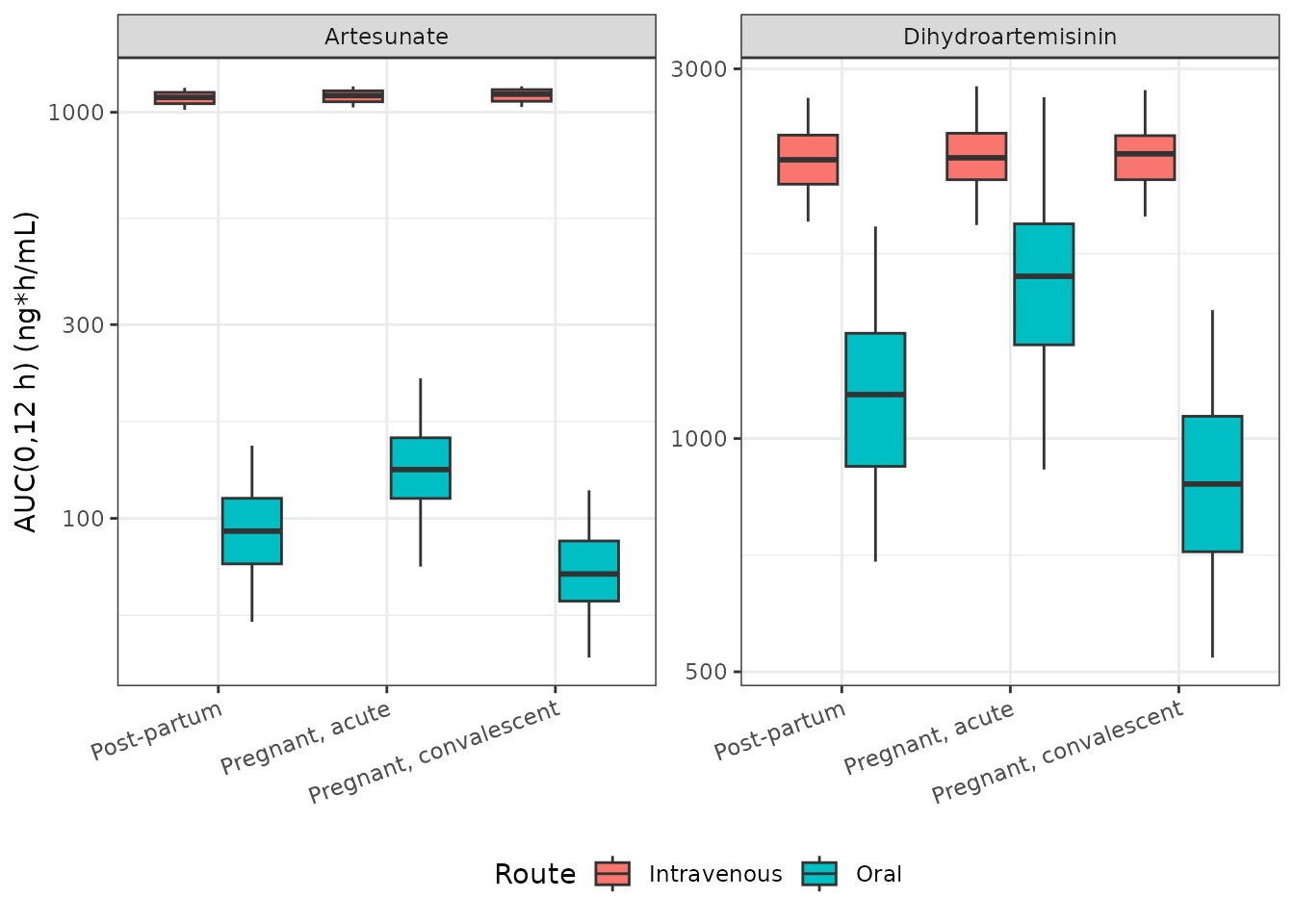

Replicates Figure 4A and 4B of Kloprogge 2015: simulated AUC(0,12 h) for artesunate and dihydroartemisinin after 4 mg/kg intravenous and oral artesunate, by phase. Boxes span the interquartile range and whiskers the 2.5th to 97.5th percentiles, as in the source figure.

The intravenous boxes are indistinguishable across the three phases for both analytes, which is the paper’s central negative result: malaria and pregnancy do not alter the disposition of parenteral artesunate. The oral boxes separate, with acute malaria the highest and pregnant convalescence the lowest.

iv_med <- exp4 |>
  filter(Route == "Intravenous") |>
  group_by(arm) |>
  summarise(m = median(auc_dha), .groups = "drop")

oral_med <- exp4 |>
  filter(Route == "Oral") |>
  group_by(arm) |>
  summarise(m = median(auc_dha), .groups = "drop")

stopifnot(
  # The intravenous arms share every parameter that matters, differing only in
  # the simulated weight range, so their medians must coincide closely.
  diff(range(iv_med$m)) / median(iv_med$m) < 0.10,
  # The oral arms must order acute > post-partum > convalescent, which is the
  # sign structure of the two covariate effects.
  oral_med$m[oral_med$arm == "Pregnant, acute"] >
    oral_med$m[oral_med$arm == "Post-partum"],
  oral_med$m[oral_med$arm == "Post-partum"] >
    oral_med$m[oral_med$arm == "Pregnant, convalescent"]
)

Dose optimisation (Figure 4C and 4D)

The paper concludes that “a 25% increase in the administered oral artesunate dose … would provide equivalent exposures during pregnancy compared with that in post-partum patients with acute uncomplicated P. falciparum malaria”. In this parameterisation that claim has an exact algebraic form: pregnancy multiplies F by 1 - 0.233 = 0.767, and exposure is proportional to F * dose, so the dose ratio restoring parity is 1 / 0.767 = 1.304. A 25% increase therefore closes the gap to 1.25 * 0.767 = 0.959, that is to within 4.1% rather than exactly.

opt_arms <- tribble(
  ~arm,                             ~PREG, ~DIS_MALARIA_ACUTE, ~ROUTE_IV, ~wt_lo, ~wt_hi, ~dose_scale,
  "Non-pregnant, 4.0 mg/kg",            0,                  1,         0,     40,     60,        1.00,
  "Pregnant, 5.0 mg/kg (+25%)",         1,                  1,         0,     40,     60,        1.25
) |>
  mutate(grp = row_number())

opt_coh <- bind_rows(lapply(seq_len(nrow(opt_arms)), function(i) {
  a <- opt_arms[i, ]
  make_cohort(a, N_PER_ARM, dose_scale = a$dose_scale)
}))

opt_exp <- solve_cohort(opt_coh, tgrid_c) |>
  left_join(opt_coh |> select(id, grp), by = "id") |>
  left_join(opt_arms |> select(grp, arm), by = "grp")

opt_med <- opt_exp |>
  group_by(arm) |>
  summarise(auc_as = median(auc_as), auc_dha = median(auc_dha), .groups = "drop")

knitr::kable(
  opt_med |>
    mutate(across(where(is.numeric), ~ round(.x, 1))) |>
    rename("Arm" = arm, "Median AUC(0,12 h), artesunate" = auc_as,
           "Median AUC(0,12 h), DHA" = auc_dha),
  caption = "Replicates Figure 4C and 4D of Kloprogge 2015. ng*h/mL."
)

Replicates Figure 4C and 4D of Kloprogge 2015. ng*h/mL.

Arm	Median AUC(0,12 h), artesunate	Median AUC(0,12 h), DHA
Non-pregnant, 4.0 mg/kg	171.6	2072.0
Pregnant, 5.0 mg/kg (+25%)	172.0	2013.2

# The typical-value ratio is exact algebra and carries no cohort randomness.
ratio_typ <- 1.25 * (1 - 0.233)
ratio_sim <- opt_med$auc_dha[opt_med$arm == "Pregnant, 5.0 mg/kg (+25%)"] /
  opt_med$auc_dha[opt_med$arm == "Non-pregnant, 4.0 mg/kg"]

cat(sprintf("Algebraic parity ratio: %.4f; simulated median ratio: %.4f\n",
            ratio_typ, ratio_sim))
#> Algebraic parity ratio: 0.9587; simulated median ratio: 0.9716

stopifnot(
  # The simulated median must track the algebra; the residual gap is the
  # cohort weight draw only, since F and dose scaling are weight-independent.
  abs(ratio_sim / ratio_typ - 1) < 0.10,
  # And the paper's qualitative claim must hold: a 25% increase brings
  # pregnant exposure within 10% of the non-pregnant reference.
  abs(ratio_sim - 1) < 0.10
)

Assumptions and deviations

• Residual-error scale. Table 2 reports four sigma values with no uncertainty and no back-transformation footnote, in the same column as the structural typical values. They are read here as NONMEM $SIGMA variance estimates, so the model file uses sqrt() of each. Three things support that reading: NONMEM reports $SIGMA as variances by default; the IIV column of the same table carries its own explicit back-transformation footnote (100 * sqrt(exp(estimate) - 1)) while the sigma rows carry none, marking them as raw estimates; and the magnitudes line up with the sibling Morris_2011_artesunate model, whose Table 2 reports the same quantity as 0.696 for artesunate and 0.174 for DHA. If they were instead standard deviations, every residual magnitude here would be roughly 8% to 20% smaller. Nothing in the validation above depends on the choice, because every exposure metric is taken from the individual predictions rather than from a residual-carrying simulated observation.
• “Additive on log-transformed data” is encoded as lnorm(), not prop(). The two are equivalent only to first order, and these residual magnitudes are far too large for that approximation: a proportional error with SD 1.077 would drive roughly 18% of simulated artesunate observations negative. The log-normal form is both the faithful reading of the paper’s sentence and the one that keeps concentrations positive.
• Inter-occasion variability is omitted. The paper estimates IOV of 60.2% CV on the first-pass fraction BIO, and no IIV on it. Packaged library models do not carry IOV (the same convention as Bukkems_2021_raltegravir and Kloprogge_2014_quinine), so fp is a deterministic typical value here. Simulated between-subject spread in artesunate exposure is therefore narrower than the paper’s, and DHA exposure is essentially unaffected because the IOV redistributes flux between the two entry routes without changing the total.
• Bioavailability can exceed 1 in a simulated cohort. F carries a 27.1% CV log-normal random effect on top of a typical value that reaches 92.2% for a non-pregnant patient with acute malaria, so a minority of simulated subjects in that condition draw F above 1, which is not physically possible. The paper does not state a bounding transform, and its Table 2 footnote applies the log-normal back-transformation uniformly to every random effect including F, so the exponential form is reproduced here as published. It affects only the non-pregnant acute arm of the dose-optimisation figure; every tightly bounded check in this vignette is run on typical values with zeroRe(), where the issue cannot arise.
• Transit-chain length. Figure 1 states ktr = (n + 1) / MTT with n = 6 fixed, so seven states - the depot plus six transit compartments - empty at ktr and an eighth empties at ka. This is the Savic-style chain with a separate absorption compartment, which is required by the model carrying both ktr and ka as distinct parameters in Table 2 and Figure 1. The resulting mean absorption time, MTT + 1/ka = 0.407 + 0.637 = 1.04 h, matches the published oral tmax of 1.00 to 1.06 h.
• Post-partum days 1-2 and day 7 are one condition. The two published columns carry identical covariate values in this model, so only one is simulated; their published difference (AUC 1050 against 1040 for DHA) is empirical-Bayes noise.
• Early artesunate is deliberately not gated tightly. The paper itself reports that “the 95th and 5th percentiles of early artesunate concentrations after intravenous and oral artesunate were substantially over and under estimated” in the visual predictive check, and attributes the misspecification below 30 minutes to erratic data. Artesunate tmax after oral dosing is predicted around 0.66 h against a published 1.00 to 1.06 h. It is reproduced, not tuned.
• Intravenous dose records must carry rate = -2. The model declares dur(central) <- dur_iv with the duration fixed at the paper’s 0.0167 h, but rxode2 only honours a modelled duration when the dose record asks for it. An intravenous record without rate = -2 is delivered as an instantaneous bolus, which raises the artesunate peak to Dose / Vc and over-predicts the published Cmax by about 18% while leaving every AUC untouched. With the infusion active the predicted peak is 16600 to 16700 ng/mL against a published 17800.
• Artesunate is flip-flop after oral dosing. ka = 1.57 /h lies below the artesunate terminal disposition rate constant lambda_z = 2.94 /h, so the terminal slope of an oral profile is set by absorption and an NCA half-life on it returns 0.441 h rather than the 0.236 h disposition half-life. Table 3 repeats one artesunate half-life across the intravenous and oral columns of each visit, so the published number is the disposition value; the oral half-life reference is therefore left blank in the comparison table above rather than being scored against a different quantity. DHA is not affected - its absorption is far faster than its 1.25 h disposition half-life - and its half-life matches to within 2.1% on every condition and both routes.
• tmax after intravenous dosing is sampling-grid limited in the source. The published DHA tmax of 0.100 h (range 0.100 to 0.200) can only take the values of the nominal intravenous sampling schedule, whose first three post-dose times are 5, 15 and 30 minutes. The model peaks at 0.145 h, that is 8.7 minutes, between the first two of those samples; the 45% relative difference is 2.7 minutes in absolute terms.
• Weight distributions are assumed uniform over the ranges the source figure legends give (39 to 64 kg pregnant, 37 to 62 kg post-partum, 40 to 60 kg for the dose optimisation). The paper reports ranges, not distributions.
• Covariate columns. DIS_MALARIA_ACUTE is registered by this extraction as a new canonical in the DIS_<condition> family. Unlike its siblings it is time-varying within subject, marking a phase of an episode rather than membership of a cohort; the _ACUTE suffix is load-bearing, because a bare DIS_MALARIA would read as false for the day-7 convalescent records that carry 0 here. ROUTE_IV uses oral, not subcutaneous, as its reference category and selects the residual magnitude only.
• Pregnancy was carried on bioavailability, not on DHA clearance. The paper reports that pregnancy on DHA elimination clearance gave a larger objective-function drop (-45.1) than pregnancy on bioavailability (-22.5), and that the two parameterisations give a similar effect size (27% against 23%). The authors nonetheless carried bioavailability forward, because covariate modelling on the intravenous data alone could not detect a pregnancy effect on clearance, in agreement with the non-compartmental analysis. The published final model is what is reproduced here.