Tacrolimus (Antignac 2007)
Source:vignettes/articles/Antignac_2007_tacrolimus.Rmd
Antignac_2007_tacrolimus.RmdModel and source
- Citation: Antignac M, Barrou B, Farinotti R, Lechat P, Urien S. Population pharmacokinetics and bioavailability of tacrolimus in kidney transplant patients. Br J Clin Pharmacol. 2007;64(6):750-757. doi:10.1111/j.1365-2125.2007.02895.x
- Article: https://doi.org/10.1111/j.1365-2125.2007.02895.x
The packaged model encodes the one-compartment final structural model from Antignac 2007 Equation p. 754 and Table 4 (Original dataset Mean column):
- first-order absorption with
kafixed at 4.5 1/h (taken from Jusko 1995 because only trough samples were available in the dataset andkawas unidentifiable from the data); - linear elimination from a single central compartment of volume
V; - oral bioavailability
Festimated from the joint analysis of IV and oral records; - a Hill-type sigmoidal recovery of clearance with days post-operation
(
POD),CL = CLmin * (1 + POD^gCL / (POD^gCL + TCL50^gCL)), that saturates atCLmax = 2 * CLminas POD becomes large; and - a multiplicative high-prednisone-dose effect on clearance,
CL = CL * (1 + theta_PRD)when the concomitant prednisone dose exceeds 25 mg/day.
Population
The source cohort was 83 adult kidney transplant recipients (54 M / 29 F) followed at Pitie-Salpetriere Hospital, Paris, between January 2003 and September 2004. Median age 46 years (range 16 - 67); median body weight 69 kg (range 29 - 100). Patients received tacrolimus as primary immunosuppressant alongside mycophenolate mofetil and corticosteroids; 25 of 83 received an initial intravenous course and were transitioned to oral dosing within 24 - 48 hours, the remaining 58 received oral dosing only. The dataset comprised 1589 trough whole-blood tacrolimus concentrations collected during the first two months post-transplantation under routine therapeutic drug monitoring (MEIA, IMx platform, LLOQ 1.5 ng/mL). Source demographics: Antignac 2007 Tables 1 and 2.
The same information is available programmatically via the model’s
population metadata
(readModelDb("Antignac_2007_tacrolimus")$population exposes
the list).
Source trace
The per-parameter origin is recorded as an in-file comment next to
each ini() entry in
inst/modeldb/specificDrugs/Antignac_2007_tacrolimus.R. The
table below collects them in one place for review.
| Equation / parameter | Value | Source location |
|---|---|---|
lcl (CLmin) |
log(1.81 L/h) | Table 4, Original dataset Mean, TV(CLmin) |
lvc (V) |
log(98.4 L) | Table 4, Original dataset Mean, V |
lfdepot (F) |
log(0.137) | Table 4, Original dataset Mean, F (13.7%) |
lka (FIXED) |
log(4.5 1/h) | Table 4, Original dataset, ka fixed; from Jusko 1995 (ref 10) |
tcl50 |
3.81 days | Table 4, Original dataset Mean, TCL50 |
gamma_cl |
2.54 | Table 4, Original dataset Mean, gCl |
e_pred_dose_high_cl (theta_PRD) |
0.575 | Table 4, Original dataset Mean, qPRD |
etalcl IIV (%CV 31%) |
log(0.31^2 + 1) | Table 4, wClmin (%) |
etalvc IIV (%CV 79%) |
log(0.79^2 + 1) | Table 4, wV (%) |
etalfdepot IIV (%CV 32%) |
log(0.32^2 + 1) | Table 4, wF (%) |
propSd (18.6%) |
0.186 | Table 4, Residual proportional variance s (%) |
addSd (0.96 ng/mL) |
0.96 | Table 4, Residual additive variance s (ng/mL) |
d/dt(depot) (first-order absorption) |
n/a | Methods, “Population pharmacokinetic modelling” (ADVAN2 TRANS2) |
d/dt(central) (linear elimination) |
n/a | Methods, “Population pharmacokinetic modelling” |
CL = CLmin * (1 + POD^gCL / (POD^gCL + TCL50^gCL)) * E_PRD |
n/a | Equation p. 754 |
E_PRD = 1 + theta_PRD when PRD > 25, else 1 |
n/a | Equation p. 754 |
f(depot) <- F (oral only) |
n/a | Methods, “Population pharmacokinetic modelling” (simultaneous IV+oral fit) |
Virtual cohort
Original observed data are not publicly available. The figures below
use virtual cohorts whose covariate distributions approximate the
published trial: typical body weight, two prednisone-dose groups
bracketing the >25 mg/day threshold (22 mg/day for the typical
maintenance group, 30 mg/day for the high-dose group), and
POD advancing one integer day per 24 hours of simulated
time, anchored to POD = 1 at the first dose per the paper’s
“POD = 1 corresponds to the transplantation date” convention.
Two multi-dose cohorts of 100 simulated subjects each carry oral tacrolimus 5 mg twice daily for 21 days (well within the published two-month follow-up window). A third single-dose cohort of 100 subjects receives a single 5 mg oral dose with dense sampling out to 72 hours for the NCA validation block.
set.seed(20070409)  # paper's "Published OnlineEarly" date as a reproducible seed

cohort_size  <- 100L                    # 100 per cohort (well under the 200 / arm cap)
dose_amt     <- 5                       # mg per oral dose
dose_tau     <- 12                      # hours between doses
n_doses      <- 42L                     # 21 days * 2 doses/day

# POD steps up by 1 every 24 simulated hours, anchored at POD = 1 at t = 0.
pod_at_time <- function(t) floor(t / 24) + 1L

make_multi_dose_events <- function(n, pred_dose_value, cohort_label, id_offset = 0L) {
  obs_times <- seq(0, dose_tau * n_doses, by = 12)
  dose_times <- seq(0, dose_tau * (n_doses - 1L), by = dose_tau)

  doses <- tidyr::expand_grid(
    id = id_offset + seq_len(n),
    time = dose_times
  ) |>
    dplyr::mutate(
      evid       = 1L,
      amt        = dose_amt,
      cmt        = "depot",
      PRED_DOSE  = pred_dose_value,
      POD        = pod_at_time(time),
      cohort     = cohort_label
    )

  obs <- tidyr::expand_grid(
    id = id_offset + seq_len(n),
    time = obs_times
  ) |>
    dplyr::mutate(
      evid       = 0L,
      amt        = NA_real_,
      cmt        = "central",
      PRED_DOSE  = pred_dose_value,
      POD        = pod_at_time(time),
      cohort     = cohort_label
    )

  dplyr::bind_rows(doses, obs) |>
    dplyr::arrange(id, time, dplyr::desc(evid))
}

make_single_dose_events <- function(n, pred_dose_value, cohort_label, id_offset = 0L) {
  obs_times <- c(seq(0, 12, by = 0.5), seq(13, 72, by = 1))

  doses <- tibble::tibble(
    id        = id_offset + seq_len(n),
    time      = 0,
    evid      = 1L,
    amt       = dose_amt,
    cmt       = "depot",
    PRED_DOSE = pred_dose_value,
    POD       = 1L,
    cohort    = cohort_label
  )

  obs <- tidyr::expand_grid(
    id = id_offset + seq_len(n),
    time = obs_times
  ) |>
    dplyr::mutate(
      evid       = 0L,
      amt        = NA_real_,
      cmt        = "central",
      PRED_DOSE  = pred_dose_value,
      POD        = 1L,
      cohort     = cohort_label
    )

  dplyr::bind_rows(doses, obs) |>
    dplyr::arrange(id, time, dplyr::desc(evid))
}

events_multi <- dplyr::bind_rows(
  make_multi_dose_events(cohort_size, pred_dose_value = 22, cohort_label = "typical_PRED_22mg",
                         id_offset =                       0L),
  make_multi_dose_events(cohort_size, pred_dose_value = 30, cohort_label = "high_PRED_30mg",
                         id_offset =              cohort_size)
)

events_nca <- make_single_dose_events(cohort_size, pred_dose_value = 22,
                                      cohort_label = "single_dose_PRED_22mg",
                                      id_offset = 2L * cohort_size)

stopifnot(!anyDuplicated(unique(events_multi[, c("id", "time", "evid")])))
stopifnot(!anyDuplicated(unique(events_nca[, c("id", "time", "evid")])))
Simulation
mod <- readModelDb("Antignac_2007_tacrolimus")

sim_multi <- rxode2::rxSolve(
  mod,
  events = events_multi,
  keep   = c("cohort", "POD", "PRED_DOSE")
) |>
  as.data.frame()

sim_nca <- rxode2::rxSolve(
  mod,
  events = events_nca,
  keep   = c("cohort", "POD", "PRED_DOSE")
) |>
  as.data.frame()
For deterministic replication (typical-value trajectories without between-subject variability), zero out the random effects:
mod_typical <- mod |> rxode2::zeroRe()

events_typ <- make_multi_dose_events(1L, pred_dose_value = 22,
                                     cohort_label = "typical_subject")

sim_typical <- rxode2::rxSolve(
  mod_typical, events = events_typ,
  keep = c("cohort", "POD", "PRED_DOSE")
) |>
  as.data.frame()
#> ℹ omega/sigma items treated as zero: 'etalcl', 'etalvc', 'etalfdepot'
Replicate published figures
Figure 1 – Tacrolimus trough concentrations vs time
Antignac 2007 Figure 1 plots the 1589 observed trough whole-blood tacrolimus concentrations against time (hours), overlaid with the median and the 2.5th / 97.5th percentiles. The simulated VPC below mirrors that plot for the typical maintenance cohort over the first 21 days (504 hours) of treatment. The shape (initial rise to a peak around POD = 3 - 5 days as CL is still in the lower half of its sigmoidal recovery, then a slow decline toward steady state) matches the published figure.
sim_multi |>
  dplyr::filter(time > 0, cohort == "typical_PRED_22mg") |>
  dplyr::group_by(time) |>
  dplyr::summarise(
    Q025 = stats::quantile(Cc, 0.025, na.rm = TRUE),
    Q50  = stats::quantile(Cc, 0.50,  na.rm = TRUE),
    Q975 = stats::quantile(Cc, 0.975, na.rm = TRUE),
    .groups = "drop"
  ) |>
  ggplot(aes(time, Q50)) +
  geom_ribbon(aes(ymin = Q025, ymax = Q975), alpha = 0.2) +
  geom_line(linewidth = 0.7) +
  labs(
    x       = "Time (hours)",
    y       = "Simulated tacrolimus trough Cc (ng/mL)",
    title   = "Figure 1 replicate (typical PRED 22 mg/day cohort, 5 mg PO BID)",
    caption = "Median (solid) and 2.5/97.5th percentile band; n = 100 simulated subjects."
  )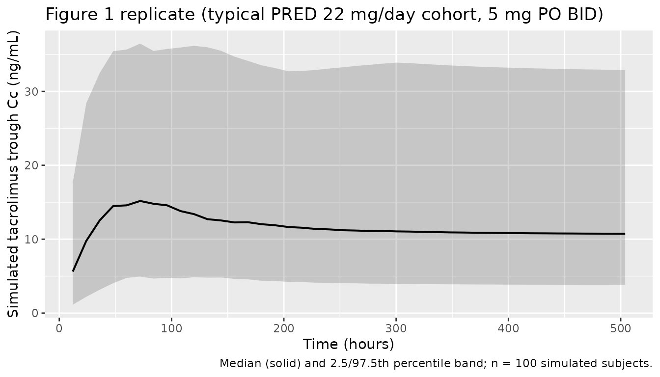
Figure 2 – Typical CL vs POD
Antignac 2007 Figure 2 shows individual clearance estimates plotted
against POD, with overlaid model-predicted lines for the
high- and low-prednisone-dose subpopulations. The simulated curves below
are constructed analytically from the packaged model: the population
typical CL as a function of POD for
PRED_DOSE = 22 mg/day (no high-dose effect) and
PRED_DOSE = 30 mg/day (high-dose effect active).
pod_grid <- seq(0, 15, length.out = 200)
tcl50     <- 3.81
gamma_cl  <- 2.54
clmin     <- 1.81
theta_prd <- 0.575

cl_by_pod <- tibble::tibble(
  POD = rep(pod_grid, times = 2L),
  cohort = rep(c("typical_PRED_22mg", "high_PRED_30mg"), each = length(pod_grid))
) |>
  dplyr::mutate(
    pod_effect  = 1 + POD^gamma_cl / (POD^gamma_cl + tcl50^gamma_cl),
    pred_effect = ifelse(cohort == "high_PRED_30mg", 1 + theta_prd, 1),
    CL          = clmin * pod_effect * pred_effect
  )

ggplot(cl_by_pod, aes(POD, CL, colour = cohort, linetype = cohort)) +
  geom_line(linewidth = 0.8) +
  scale_colour_brewer(palette = "Set1") +
  labs(
    x       = "Post-operative day, POD (days)",
    y       = "Population typical CL (L/h)",
    colour  = "Prednisone cohort",
    linetype = "Prednisone cohort",
    title   = "Figure 2 replicate -- typical CL as a function of POD",
    caption = "Drawn analytically from the packaged ini() parameters (CLmin = 1.81 L/h, TCL50 = 3.81 d, gCL = 2.54, theta_PRD = 0.575)."
  )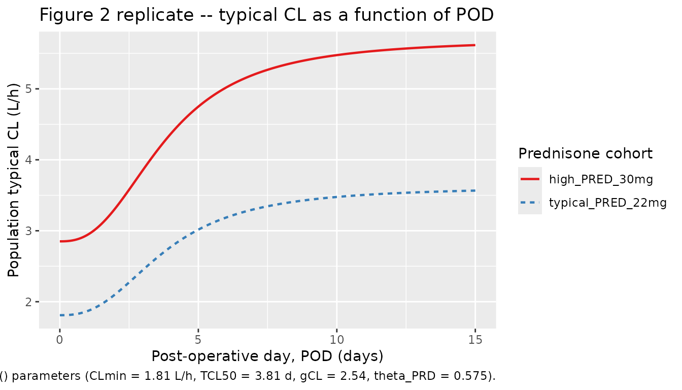
The PRED effect doubles the asymptote separation visible at large
POD in the published figure:
CLmax_high / CLmax_typical = 1 + theta_PRD = 1.575,
i.e. about 60% higher CL in the high-prednisone subpopulation.
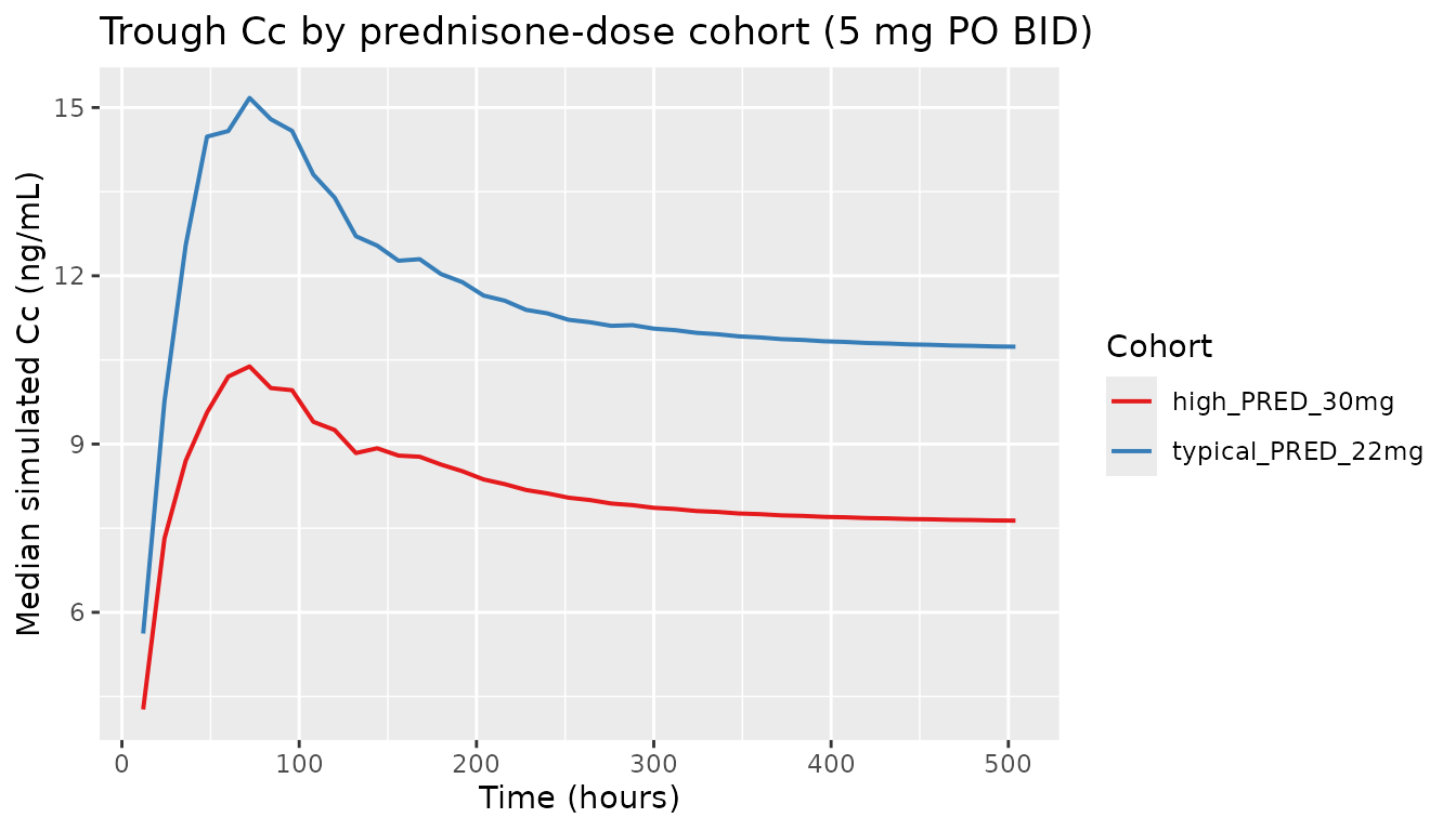
Comparing the two cohorts at steady state
The high-prednisone cohort reaches lower steady-state troughs because of the boosted clearance. Both cohorts use the same 5 mg PO BID regimen.
sim_multi |>
  dplyr::filter(time > 0) |>
  dplyr::group_by(cohort, time) |>
  dplyr::summarise(Q50 = stats::quantile(Cc, 0.5, na.rm = TRUE), .groups = "drop") |>
  ggplot(aes(time, Q50, colour = cohort)) +
  geom_line(linewidth = 0.7) +
  scale_colour_brewer(palette = "Set1") +
  labs(
    x      = "Time (hours)",
    y      = "Median simulated Cc (ng/mL)",
    colour = "Cohort",
    title  = "Trough Cc by prednisone-dose cohort (5 mg PO BID)"
  )
PKNCA validation
The paper does not report subject-level NCA parameters (it reports
popPK estimates only), so the comparison below pairs PKNCA-derived NCA
from a single-dose simulation against analytical expectations computed
from the packaged ini() values (Cmax, Tmax, AUC0-inf,
half-life under the one-compartment first-order absorption model). A
close match between the two columns confirms that the packaged
structural model and the encoded parameter values together reproduce the
equations and numbers in the source paper. The analytical expectations
use the PRED_DOSE = 22 mg/day low-prednisone branch at
POD = 1, which gives a population typical
CL(POD = 1) = CLmin * (1 + 1 / (1 + TCL50^gCL)).
sim_nca_pknca <- sim_nca |>
  dplyr::filter(!is.na(Cc)) |>
  dplyr::select(id, time, Cc, cohort)

sim_nca_pknca <- dplyr::bind_rows(
  sim_nca_pknca,
  sim_nca_pknca |> dplyr::distinct(id, cohort) |>
    dplyr::mutate(time = 0, Cc = 0)
) |>
  dplyr::distinct(id, cohort, time, .keep_all = TRUE) |>
  dplyr::arrange(id, cohort, time)

conc_obj <- PKNCA::PKNCAconc(sim_nca_pknca, Cc ~ time | cohort + id)

dose_df <- events_nca |>
  dplyr::filter(evid == 1L) |>
  dplyr::select(id, time, amt, cohort)

dose_obj <- PKNCA::PKNCAdose(dose_df, amt ~ time | cohort + id)

intervals <- data.frame(
  start      = 0,
  end        = Inf,
  cmax       = TRUE,
  tmax       = TRUE,
  aucinf.obs = TRUE,
  half.life  = TRUE
)

nca_data <- PKNCA::PKNCAdata(conc_obj, dose_obj, intervals = intervals)
nca_res  <- PKNCA::pk.nca(nca_data)
Comparison against analytical expectations
# Analytical one-compartment first-order absorption (oral) expectations at
# POD = 1, PRED_DOSE = 22 mg/day (no high-dose boost).
cl_at_pod1 <- clmin * (1 + 1^gamma_cl / (1^gamma_cl + tcl50^gamma_cl))   # L/h
v   <- 98.4                                                              # L
f   <- 0.137                                                             # fraction
ka  <- 4.5                                                               # 1/h
dose <- 5                                                                # mg

kel       <- cl_at_pod1 / v
tmax_an   <- log(ka / kel) / (ka - kel)
cmax_an   <- f * dose * ka / (v * (ka - kel)) *
             (exp(-kel * tmax_an) - exp(-ka * tmax_an)) * 1000           # ng/mL
aucinf_an <- f * dose / cl_at_pod1 * 1000                                # ng h / mL
thalf_an  <- log(2) / kel                                                # hours

expected <- tibble::tibble(
  cohort     = "single_dose_PRED_22mg",
  cmax       = cmax_an,
  tmax       = tmax_an,
  aucinf.obs = aucinf_an,
  half.life  = thalf_an
)

cmp <- nlmixr2lib::ncaComparisonTable(
  simulated     = nca_res,
  reference     = expected,
  by            = "cohort",
  units         = c(cmax = "ng/mL", aucinf.obs = "ng*h/mL",
                    tmax = "h", half.life = "h"),
  tolerance_pct = 20
)

knitr::kable(
  cmp,
  caption = paste(
    "Simulated NCA vs analytical first-order-absorption expectations at",
    "POD = 1, PRED_DOSE = 22 mg/day. * differs from reference by >20%."
  ),
  align = c("l", "l", "r", "r", "r")
)| NCA parameter | cohort | Reference | Simulated | % diff |
|---|---|---|---|---|
| Cmax (ng/mL) | single_dose_PRED_22mg | 6.8 | 5.63 | -17.2% |
| Tmax (h) | single_dose_PRED_22mg | 1.22 | 1.5 | +22.9%* |
| AUC0-∞ (obs) (ng*h/mL) | single_dose_PRED_22mg | 367 | 370 | +0.8% |
| t½ (h) | single_dose_PRED_22mg | 36.5 | 39.7 | +8.7% |
Assumptions and deviations
- The paper’s abstract and Discussion section state
Vin units of L/kg (“typical value for volume of distribution, V, (98 +/- 13 l kg-1)”), while Table 4 listsV (l)with mean 98.4 L and the bootstrap 2.5 - 97.5th percentile range 56.4 - 273 L. We use the Table 4 value (V = 98.4 L total) because the bootstrap percentile range is consistent with L total at this population’s body-weight distribution and is inconsistent with L/kg (which would imply 6800 L for a 70 kg adult and a percentile range of 3900 - 19000 L). The “L kg-1” qualifier in the abstract / Discussion appears to be a unit typo. - Prednisone-dose units. Antignac 2007 Methods records the prednisone
covariate as “prednisone (mg) (PRD)” without specifying mg/day vs.
mg/dose. We adopt the daily-dose interpretation (mg/day) consistent with
the transplant-immunosuppressant tapering schedule referenced in the
Discussion (“After surgery, patients received intravenous
methylprednisolone and 2 or 3 days later were transferred to oral
prednisone at an initial dose of 30 mg which could be decreased by steps
of 2.5 mg according to clinical parameters”) and with the registered
canonical
PRED_DOSE(mg/day). The 25 mg/day threshold in the model is then a daily-dose threshold. -
POD = 1anchor. The paper statesPOD = 1corresponds to the transplantation date. To avoid evaluatingPOD^gamma_clatPOD = 0in the recovery curve (numerically0^2.54 = 0, which makes the bracket equal to 1 = the correct CLmin limit but can be sensitive to rounding in some implementations), the vignette anchors simulations atPOD = 1attime = 0, matching the paper’s convention exactly. The ODE-state andf(depot)definitions remain unchanged. -
kais held fixed at 4.5 1/h in the source paper (taken from Jusko 1995 because only trough samples were available in the cohort andkawas unidentifiable). The packaged model preserves thisfixed()status to make the provenance explicit; downstream users who want to re-estimatekaagainst a richer dataset must remove thefixed()wrapper. - IIV on
Fis encoded with the paper’s stated exponential form (F_i = TV(F) * exp(eta_F)), which can in principle yieldF_i > 1. The reportedomega_F(32% CV) combined with the typical valueF = 0.137keeps the implied right tail well below 1 in practice (the bootstrap 2.5 - 97.5th percentile range in Table 4 is 6.4 - 22.9 %, all below 100%); a logit transform was not used because the source paper’s encoding is exponential and a logit reparameter- isation would deviate from the published model. - No NCA values are reported in the source paper for direct comparison, so the validation table compares simulated NCA against analytical expectations derived from the packaged structural model and parameter values rather than against transcribed published numbers.