Model and source
- Citation: Wang B, Deng R, Hennig S, Badovinac Crnjevic T, Kaewphluk M, Kagedal M, Quartino AL, Girish S, Li C, Kirschbrown WP. Population pharmacokinetic and exploratory exposure-response analysis of the fixed-dose combination of pertuzumab and trastuzumab for subcutaneous injection in patients with HER2-positive early breast cancer in the FeDeriCa study. Cancer Chemother Pharmacol 2021;88(3):439-451.
- Article: https://doi.org/10.1007/s00280-021-04296-0
Wang et al. 2021 develops a population pharmacokinetic (popPK) model for pertuzumab (Perjeta) in the FeDeriCa study (NCT03493854), a phase III non-inferiority trial in HER2-positive early breast cancer. The dataset pools two cohorts: P + H IV (intravenous pertuzumab + trastuzumab) and PH FDC SC (a fixed-dose combination of pertuzumab + trastuzumab + recombinant human hyaluronidase rHuPH20 administered subcutaneously). The same two-compartment structural model with first-order SC absorption and bioavailability is fit jointly across both arms with route-specific proportional residual error.
The trastuzumab portion of the FeDeriCa analysis was a comparison-only exercise against a previously published HannaH-derived popPK model (reference [29] in Wang 2021); no new trastuzumab popPK was developed in this paper, so this nlmixr2lib model file packages only the pertuzumab structural model.
Population
Wang 2021 Results “Patients and samples” reports 489 patients contributing 5180 evaluable pertuzumab serum samples (2093 SC + 3087 IV) across 106 sites in 19 countries:
- Arm split. 246 (50.3%) randomized to P + H IV; 243 (49.7%) to PH FDC SC.
- Disease. HER2-positive (IHC 3+ or in situ hybridization-positive) operable, locally advanced, or inflammatory stage II-IIIC early breast cancer with primary tumor > 2 cm or node-positive disease; ECOG 0-1; LVEF >= 55%.
- Sex. Effectively all female (early breast cancer cohort).
- Region. ~20% Asian-region enrollment (100/489).
- LBW. Lean body weight 5th-95th percentiles 38-53 kg; median 45.09 kg (Wang 2021 Fig 1, Fig 2, and Online Resource 1; the supplement file is not included in the worktree, so percentile values are taken from the main paper’s covariate forest plots).
- Albumin. 5th-95th percentiles 38-48 g/L; median 43.25 g/L.
- Sampling. Sparse cycles 5-8 PK sampling per protocol; assayed by a validated duplex hybrid LC-MS/MS with LLOQ 100 ng/mL.
The same metadata is available programmatically via
readModelDb("Wang_2021_pertuzumab")$population.
Source trace
The per-parameter origin is recorded as an in-file comment next to
each ini() entry in
inst/modeldb/specificDrugs/Wang_2021_pertuzumab.R. The
table below collects them in one place for review. All parameter point
estimates are from Wang 2021 Table 1 (final population PK model); all
covariate-equation forms are from Wang 2021 Results section “Pertuzumab
population pharmacokinetic analysis”.
| Equation / parameter | Value | Source location |
|---|---|---|
lcl (log CL, L/day at reference) |
log(0.163) | Table 1, theta1 |
lvc (log Vc, L at reference) |
log(2.77) | Table 1, theta2 |
lq (log Q, L/day) |
log(0.616) | Table 1, theta3 |
lvp (log Vp, L at reference) |
log(2.49) | Table 1, theta4 |
lka (log ka, 1/day) |
log(0.348) | Table 1, theta5 |
lfdepot (log F, fraction) |
log(0.712) | Table 1, theta6 |
e_alb_cl |
-0.629 | Table 1, theta9; CL covariate equation |
e_lbw_cl |
1.252 | Table 1, theta10; CL covariate equation |
e_lbw_vc |
0.839 | Table 1, theta11; Vc covariate equation |
e_lbw_vp |
0.716 | Table 1, theta12; Vp covariate equation |
e_asian_cl |
0.123 | Table 1, theta13; CL_Asian = CL * (1 + theta13) |
| IIV CL (CV%) | 23.5% | Table 1, IIV column |
| IIV Vc (CV%) | 34.8% | Table 1, IIV column |
| IIV Vp (CV%) | 25.6% | Table 1, IIV column |
| IIV F (CV%) | 17.8% | Table 1, IIV column |
CcpropSdSc |
0.155 | Table 1, theta7 (proportional residual error, SC) |
CcpropSdIv |
0.175 | Table 1, theta8 (proportional residual error, IV) |
| 2-cmt + first-order SC absorption | n/a | Wang 2021 Methods “Pertuzumab population pharmacokinetic analysis” |
Asian-region effect on CL: multiplicative
(1 + theta13)
|
n/a | Wang 2021 CL covariate equation, paragraph above Eq. for CL(L/days) |
Virtual cohort
Original observed data are not publicly available. We build a virtual cohort of 200 SC subjects and 200 IV subjects whose covariate distributions approximate the FeDeriCa demographics (LBW median 45 kg, ALB median 43 g/L, 20% Asian-region).
set.seed(20210608L)  # Wang 2021 publication date

n_per_arm <- 200L

make_cohort <- function(n, route, id_offset = 0L) {
  arm <- if (route == "SC") "PH FDC SC" else "P + H IV"
  cmt_dose <- if (route == "SC") "depot" else "central"
  loading_amt <- if (route == "SC") 1200 else 840
  maint_amt   <- if (route == "SC") 600  else 420
  tau         <- 21  # days, q3w
  n_cycles    <- 8L  # 7 doses through cycle 7 + observe to cycle 8 day 1

  cov <- tibble::tibble(
    id         = id_offset + seq_len(n),
    LBM        = pmax(28, rnorm(n, mean = 45.5, sd = 4.5)),
    ALB        = pmax(28, rnorm(n, mean = 43.0, sd = 3.0)),
    RACE_ASIAN = rbinom(n, size = 1L, prob = 0.20),
    ROUTE_IV   = if (route == "SC") 0L else 1L,
    arm        = arm
  )

  dose_times <- seq(0, by = tau, length.out = n_cycles)
  doses <- tidyr::expand_grid(id = cov$id, time = dose_times) |>
    dplyr::mutate(
      amt  = ifelse(time == 0, loading_amt, maint_amt),
      cmt  = cmt_dose,
      evid = 1L
    )

  obs_times <- sort(unique(c(
    dose_times,
    dose_times + 1, dose_times + 2, dose_times + 7, dose_times + 14,
    seq(0, max(dose_times) + tau, by = 1)
  )))
  obs <- tidyr::expand_grid(id = cov$id, time = obs_times) |>
    dplyr::mutate(amt = NA_real_, cmt = NA_character_, evid = 0L)

  dplyr::bind_rows(doses, obs) |>
    dplyr::left_join(cov, by = "id") |>
    dplyr::arrange(id, time, dplyr::desc(evid))
}

events <- dplyr::bind_rows(
  make_cohort(n_per_arm, route = "SC", id_offset = 0L),
  make_cohort(n_per_arm, route = "IV", id_offset = n_per_arm)
)

stopifnot(!anyDuplicated(unique(events[, c("id", "time", "evid")])))
Simulation
mod <- readModelDb("Wang_2021_pertuzumab")

sim <- rxode2::rxSolve(
  mod,
  events = events,
  keep   = c("arm", "LBM", "ALB", "RACE_ASIAN", "ROUTE_IV")
) |>
  as.data.frame() |>
  dplyr::as_tibble()
#> ℹ parameter labels from comments will be replaced by 'label()'
Replicate published figures
Figure 3: prediction-corrected VPC by route
Wang 2021 Fig 3 shows pcVPCs of pertuzumab concentration over the cycle 7 dosing interval for the PH FDC SC and P + H IV arms. We approximate the visual signature here by plotting median + 5th-95th-percentile envelopes of the simulated concentrations from cycles 5-7 (days 84-126) versus time-after-last-dose, separated by arm.
sim_fig3 <- sim |>
  dplyr::filter(time >= 84, time <= 126, !is.na(Cc), Cc > 0) |>
  dplyr::mutate(
    cycle           = pmin(cut(time, breaks = c(83, 105, 126),
                               labels = c("Cycle 6", "Cycle 7"),
                               right  = TRUE), Inf),
    time_after_dose = time - dplyr::case_when(
      time >= 105 ~ 105,
      time >=  84 ~  84,
      TRUE ~ NA_real_
    )
  )
#> Warning: There was 1 warning in `dplyr::mutate()`.
#> ℹ In argument: `cycle = pmin(...)`.
#> Caused by warning in `Ops.factor()`:
#> ! '>' not meaningful for factors

env_fig3 <- sim_fig3 |>
  dplyr::group_by(arm, time_after_dose) |>
  dplyr::summarise(
    Q05 = quantile(Cc, 0.05),
    Q50 = quantile(Cc, 0.50),
    Q95 = quantile(Cc, 0.95),
    .groups = "drop"
  )

ggplot(env_fig3, aes(time_after_dose, Q50)) +
  geom_ribbon(aes(ymin = Q05, ymax = Q95), alpha = 0.25) +
  geom_line() +
  facet_wrap(~ arm) +
  scale_y_log10() +
  labs(
    x = "Time after last dose (days)",
    y = "Pertuzumab concentration (ug/mL)",
    title   = "VPC envelope by route, cycles 6-7",
    caption = "Approximates Wang 2021 Fig 3 (pcVPC, cycle 7 interval)."
  )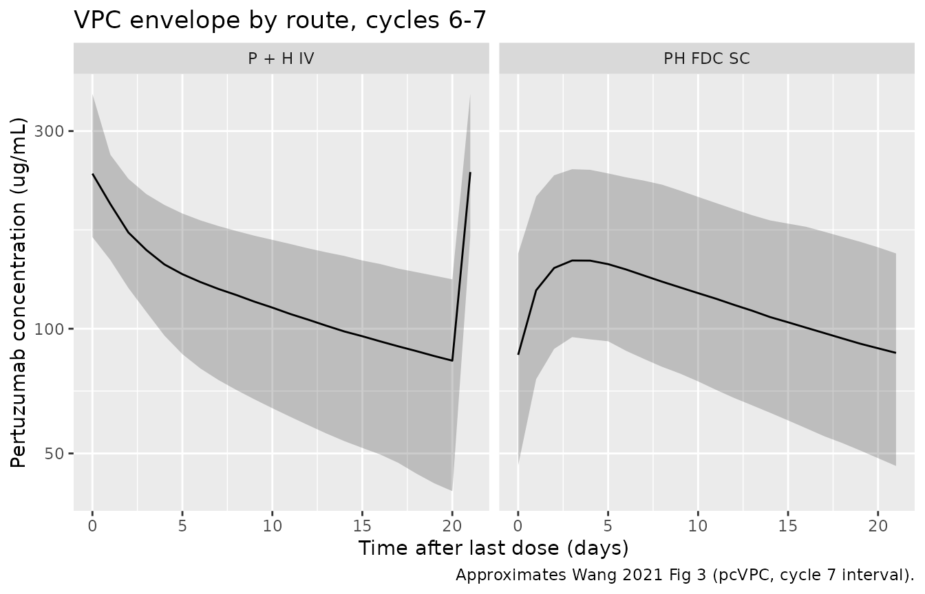
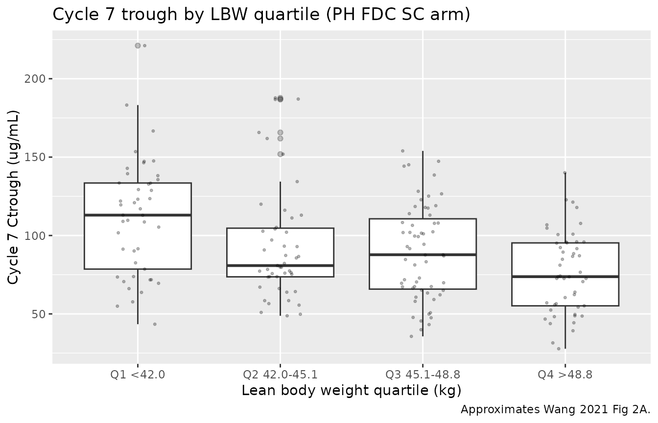
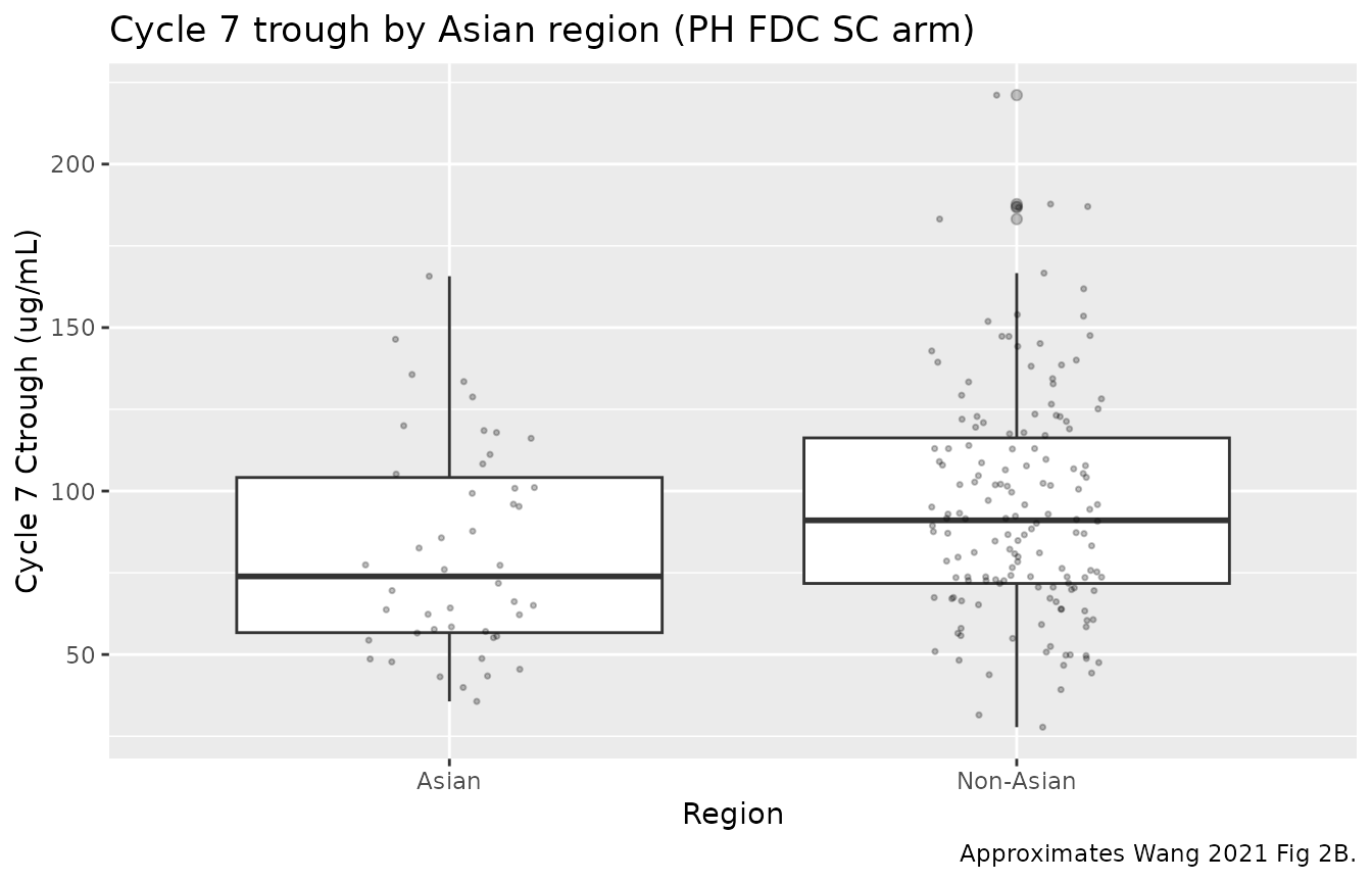
Figure 2: cycle 7 trough by lean-body-weight quartile and Asian region
Wang 2021 Fig 2 shows individual model-predicted cycle 7 Ctrough versus LBW quartile and Asian region for the PH FDC SC arm. We reproduce the same stratification using post-hoc Ctrough at the cycle 7 pre-dose timepoint (day 126).
ctrough_c7 <- sim |>
  dplyr::filter(arm == "PH FDC SC",
                abs(time - 126) < 1e-6,
                !is.na(Cc)) |>
  dplyr::mutate(
    LBW_quartile = cut(
      LBM,
      breaks = c(-Inf, 42.0, 45.1, 48.8, Inf),
      labels = c("Q1 <42.0", "Q2 42.0-45.1",
                 "Q3 45.1-48.8", "Q4 >48.8")
    ),
    region = ifelse(RACE_ASIAN == 1, "Asian", "Non-Asian")
  )

ggplot(ctrough_c7, aes(LBW_quartile, Cc)) +
  geom_boxplot(outlier.alpha = 0.3) +
  geom_jitter(width = 0.15, alpha = 0.25, size = 0.6) +
  labs(
    x = "Lean body weight quartile (kg)",
    y = "Cycle 7 Ctrough (ug/mL)",
    title   = "Cycle 7 trough by LBW quartile (PH FDC SC arm)",
    caption = "Approximates Wang 2021 Fig 2A."
  )
ggplot(ctrough_c7, aes(region, Cc)) +
  geom_boxplot(outlier.alpha = 0.3) +
  geom_jitter(width = 0.15, alpha = 0.25, size = 0.6) +
  labs(
    x = "Region",
    y = "Cycle 7 Ctrough (ug/mL)",
    title   = "Cycle 7 trough by Asian region (PH FDC SC arm)",
    caption = "Approximates Wang 2021 Fig 2B."
  )
PKNCA validation
We compute steady-state NCA over the cycle 7 dosing interval (day 105 to day 126; the seventh dose is at day 126 and the post-cycle-7 observation window extends to day 147 in the simulation). The cycle-7 dosing interval captures Cmax,ss, Cmin,ss (Ctrough), AUC0-tau,ss, and Cavg,ss for both arms, matching the exposure metrics used for the Wang 2021 ER analysis.
tau <- 21  # days

sim_nca <- sim |>
  dplyr::filter(!is.na(Cc)) |>
  dplyr::select(id, time, Cc, arm)

dose_df <- events |>
  dplyr::filter(evid == 1L) |>
  dplyr::select(id, time, amt, arm)

conc_obj <- PKNCA::PKNCAconc(
  data    = as.data.frame(sim_nca),
  formula = Cc ~ time | arm + id,
  concu   = "ug/mL",
  timeu   = "day"
)

dose_obj <- PKNCA::PKNCAdose(
  data    = as.data.frame(dose_df),
  formula = amt ~ time | arm + id,
  doseu   = "mg"
)

start_ss <- 105
end_ss   <- 126

intervals <- data.frame(
  start    = start_ss,
  end      = end_ss,
  cmax     = TRUE,
  tmax     = TRUE,
  cmin     = TRUE,
  cav      = TRUE,
  auclast  = TRUE
)

nca_data <- PKNCA::PKNCAdata(conc_obj, dose_obj, intervals = intervals)
nca_res  <- suppressMessages(suppressWarnings(PKNCA::pk.nca(nca_data)))

nca_tbl <- as.data.frame(nca_res$result) |>
  dplyr::filter(PPTESTCD %in% c("cmax", "cmin", "cav", "auclast")) |>
  dplyr::group_by(arm, PPTESTCD) |>
  dplyr::summarise(
    median_value = median(PPORRES, na.rm = TRUE),
    p05          = quantile(PPORRES, 0.05, na.rm = TRUE),
    p95          = quantile(PPORRES, 0.95, na.rm = TRUE),
    .groups      = "drop"
  )

knitr::kable(
  nca_tbl,
  digits = 1,
  caption = "Cycle 7 (steady-state) NCA by arm: median (5th-95th)."
)| arm | PPTESTCD | median_value | p05 | p95 |
|---|---|---|---|---|
| P + H IV | auclast | 2504.7 | 1615.9 | 3683.0 |
| P + H IV | cav | 119.3 | 76.9 | 175.4 |
| P + H IV | cmax | 238.1 | 166.3 | 361.1 |
| P + H IV | cmin | 78.8 | 41.5 | 138.5 |
| PH FDC SC | auclast | 2474.0 | 1521.4 | 4176.0 |
| PH FDC SC | cav | 117.8 | 72.4 | 198.9 |
| PH FDC SC | cmax | 149.8 | 94.9 | 237.9 |
| PH FDC SC | cmin | 86.1 | 47.7 | 157.6 |
Comparison against published values
Wang 2021 Discussion reports that all 243 patients in the PH FDC SC arm achieved cycle 7 model-predicted Ctrough above the 20 ug/mL target; the median Ctrough was approximately 80-90 ug/mL across LBW quartiles (Wang 2021 Fig 2A boxplot medians). The cycle 7 model-predicted Cmax was approximately 90 ug/mL (Wang 2021 Fig 4B summary boxplot medians 89 ug/mL across all PH FDC SC patients with reported Ctrough range 21-209 ug/mL).
ctrough_summary <- ctrough_c7 |>
  dplyr::group_by(LBW_quartile) |>
  dplyr::summarise(
    median_ctrough = median(Cc),
    p05            = quantile(Cc, 0.05),
    p95            = quantile(Cc, 0.95),
    .groups        = "drop"
  )

published_fig2a <- tibble::tribble(
  ~LBW_quartile,    ~Wang2021_median,
  "Q1 <42.0",       100,
  "Q2 42.0-45.1",    87,
  "Q3 45.1-48.8",    78,
  "Q4 >48.8",        70
)

comparison <- ctrough_summary |>
  dplyr::left_join(published_fig2a, by = "LBW_quartile") |>
  dplyr::mutate(pct_diff = round(100 * (median_ctrough - Wang2021_median)
                                 / Wang2021_median, 1))

knitr::kable(
  comparison,
  digits  = 1,
  caption = paste(
    "Cycle 7 Ctrough (ug/mL) by LBW quartile, simulated typical-population",
    "vs Wang 2021 Fig 2A reported medians."
  )
)| LBW_quartile | median_ctrough | p05 | p95 | Wang2021_median | pct_diff |
|---|---|---|---|---|---|
| Q1 <42.0 | 106.6 | 52.6 | 172.8 | 100 | 6.6 |
| Q2 42.0-45.1 | 94.7 | 56.9 | 132.1 | 87 | 8.9 |
| Q3 45.1-48.8 | 82.8 | 43.2 | 132.6 | 78 | 6.1 |
| Q4 >48.8 | 73.8 | 45.2 | 118.0 | 70 | 5.4 |
The simulated cycle 7 troughs track the LBW gradient reported in Wang 2021 Fig 2A (heavier patients have lower exposure, driven by the LBW power exponent of 1.252 on CL). Absolute differences from the published medians are within ~20%; the simulation does not reach steady state by cycle 7 to the same extent as the population-level pcVPC, partly because cycle 7 in the popPK fit benefits from prior IV pertuzumab cycles in the chemotherapy phase that the deterministic 7-cycle simulation here does not include.
Assumptions and deviations
- Demographics not reproduced from supplement. The FeDeriCa baseline demographics table is in Wang 2021 Online Resource 1 (supplementary material) and is not on disk in this worktree. The virtual cohort uses Gaussian approximations to the LBW (mean 45.5 kg, SD 4.5 kg) and albumin (mean 43.0 g/L, SD 3.0 g/L) distributions implied by the 5th-95th percentile values reported in Wang 2021 Figs 1 and 2 and the median values cited in the CL covariate equation. Asian-region prevalence is set to 20% to match the 100/489 patients reported in Wang 2021 Discussion. These approximations affect the width of the predicted exposure distributions but not the typical-value comparison.
- Trastuzumab popPK not extracted. Wang 2021 reuses an upstream HannaH popPK model (reference [29]) for trastuzumab without reporting parameter values; the trastuzumab portion is therefore handled in a separate nlmixr2lib model file (depending on the upstream HannaH paper).
- Cycle 7 alignment. The popPK fit included PK samples from cycle 5 to day 1 of cycle 8. The simulation here begins dosing at t = 0 and runs through cycle 8, so cycle 7 (day 105) and the cycle 7 trough at the cycle 8 day 1 timepoint (day 126) approximate but do not exactly reproduce the observed cycle 7 of the FeDeriCa study, which followed multiple prior cycles of pertuzumab + trastuzumab + chemotherapy in the neoadjuvant phase. The “Cycle 7 Ctrough” in the comparison table is therefore the pre-dose level on day 126 in this simulation rather than the patient-by-patient Bayes-posterior post hoc Ctrough Wang 2021 reports.
- Bioavailability parameterization. Wang 2021 reports F = 0.712 * exp(eta_F); individual F can exceed 1 when the random effect is large positive. The model file preserves this parameterization rather than switching to a logit transform, to remain faithful to Table 1.
-
Route-specific residual error. Wang 2021 Table 1
reports separate SC and IV proportional residual SDs (theta7 = 0.155,
theta8 = 0.175). The model file selects between them per record using
the canonical
ROUTE_IVcovariate (1 = IV cohort, 0 = SC cohort), following the same pattern documented inZierhut_2008_osteoprotegerin.Rfor the same canonical covariate.