Isavuconazole (Arrieta 2021)
Source:vignettes/articles/Arrieta_2021_isavuconazole.Rmd
Arrieta_2021_isavuconazole.RmdModel and source
- Citation: Arrieta AC, Neely M, Day JC, Rheingold SR, Sue PK, Muller WJ, Danziger-Isakov LA, Chu J, Yildirim I, McComsey GA, Frangoul HA, Chen TK, Statler VA, Steinbach WJ, Yin DE, Hamed K, Jones ME, Lademacher C, Desai A, Micklus K, Phillips DL, Kovanda LL, Walsh TJ. Safety, Tolerability, and Population Pharmacokinetics of Intravenous and Oral Isavuconazonium Sulfate in Pediatric Patients. Antimicrobial Agents and Chemotherapy. 2021;65(8):e00290-21. doi:10.1128/AAC.00290-21
- Description: Three-compartment population PK model for isavuconazole (administered as the prodrug isavuconazonium sulfate) in immunocompromised children aged 1 to <18 years pooled with adults from a phase 1 intravenous study (Arrieta 2021). Zero-order (1-h intravenous infusion) and first-order (oral capsule) input into the central compartment, linear elimination, and allometric body-weight scaling (reference 70 kg) on all clearances and volumes; no other covariates retained.
- Article: https://doi.org/10.1128/AAC.00290-21 (open access, CC BY 4.0)
- Supplement (Table S2 parameter estimates, Figure S2 goodness of fit): available from the article landing page.
Arrieta 2021 is the first pediatric study of isavuconazole, given as the water-soluble prodrug isavuconazonium sulfate. The population PK model pooled the pediatric intravenous and oral data with intravenous data from an adult phase 1 study. It was then used to simulate steady-state exposure (AUCss) for each age cohort and route and to estimate the proportion of children within the adult-derived target range of 60 to 233 ug*h/mL.
Population
Of 49 enrolled patients, 46 received study drug (safety analysis set) and 45 contributed at least one plasma concentration (PK analysis set; 551 samples: 333 intravenous, 218 oral). The intravenous cohorts were aged 1 to <6 (n = 9), 6 to <12 (n = 8) and 12 to <18 years (n = 10). The oral cohorts were aged 6 to <12 (n = 9) and 12 to <18 years (n = 10); children under 6 were excluded from the oral cohorts because of the capsule size. Across the safety set, 37% of patients were female and 72% were White. Median weight was 15.6 kg (range 10.9-19.1), 32.7 kg (18.6-67.4) and 65.9 kg (42.4-103.5) in the three intravenous cohorts, and 26.8 kg (18.3-50.1) and 50.4 kg (37.9-92.8) in the two oral cohorts (Arrieta 2021 Table 1). Patients were immunocompromised, mostly with acute leukemia, neuroblastoma or aplastic anemia, and were receiving antifungal prophylaxis. The adult data came from the phase 1 renal-impairment study of Townsend 2017 (Eur J Clin Pharmacol 73:669-678); the paper does not report how many adults were included.
All patients received isavuconazonium sulfate 10 mg/kg (maximum 372 mg) every 8 h for 6 doses, then once daily. The 372-mg cap applied above 37 kg for the 1-h intravenous infusion and above 32 kg for the 74.5-mg oral capsule (Methods, ‘Dose selection and treatment’).
| field | value | |
|---|---|---|
| species | species | human |
| n_subjects | n_subjects | 45 |
| n_studies | n_studies | 2 |
| age_range | age_range | 1-17 years (pediatric cohorts); adults from a phase 1 intravenous study (demographics not reported in this paper) |
| age_median | age_median | 10.0 years (i.v. cohort), 12.0 years (oral cohort) |
| weight_range | weight_range | 10.9-103.5 kg (pediatric) |
| weight_median | weight_median | 33.7 kg (i.v. cohort), 42.6 kg (oral cohort) |
| sex_female_pct | sex_female_pct | 37 |
| race_ethnicity | race_ethnicity | White 71.7; Black 10.9; Asian 6.5; American Indian or Alaska native 2.2; Pacific Islander 2.2; Other 6.5 |
| disease_state | disease_state | Immunocompromised children at risk for invasive mycoses (mainly acute myeloid / lymphoblastic leukemia, neuroblastoma and other solid tumors, aplastic anemia; 15% prior hematopoietic stem cell transplant) receiving antifungal prophylaxis. |
| dose_range | dose_range | Isavuconazonium sulfate 10 mg/kg (maximum 372 mg; = 5.38 mg/kg or maximum 200 mg isavuconazole) q8h for 6 doses then once daily for up to 26 days; i.v. as a 1-h infusion (1 to <18 years; 372 mg above 37 kg) or orally as 74.5-mg capsules (6 to <18 years; 372 mg above 32 kg). |
| regions | regions | United States (11 i.v. and 12 oral centers) |
| n_observations | n_observations | 551 pediatric plasma samples (333 i.v., 218 oral) plus adult i.v. data |
| notes | notes | Pediatric PK analysis set: 26 i.v. (9 aged 1 to <6, 8 aged 6 to <12, 9 aged 12 to <18 years) and 19 oral (9 aged 6 to <12, 10 aged 12 to <18 years) patients (Arrieta 2021 Table 1, Table 2; NCT03241550). Pooled with i.v. data from the adult phase 1 renal-impairment study of Townsend 2017 (Eur J Clin Pharmacol 73:669-678); adult numbers are not reported in this paper. Sex and race percentages are over the 46-patient safety analysis set (Table 1). Estimation in NONMEM with PsN 4.7.0; LLOQ 100 ng/mL. |
Source trace
Every ini() value carries an in-file comment pointing to
its source. The table collects them in one place.
| Equation / parameter | Value | Source location |
|---|---|---|
| Structure: 3 compartments, zero-order + first-order input, linear elimination | n/a | Abstract; Results, ‘Population PK model analysis’ |
lcl (CL) |
log(2.55 L/h) | Table S2 |
lvc (V2) |
log(17.80 L) | Table S2 |
lq (Q3) |
log(30.30 L/h) | Table S2 |
lvp (V3) |
log(26.00 L) | Table S2 |
lq2 (Q4) |
log(24.50 L/h) | Table S2 |
lvp2 (V4) |
log(254.0 L) | Table S2 |
lka (Ka) |
log(0.162 1/h) | Table S2 (unit printed as ‘h’) |
lfdepot (F1) |
log(0.95) | Table S2 |
e_wt_cl_q |
0.75 (fixed) | Methods allometric equation
P_ped = P_adult * (WT/70)^x; x not printed, conventional
value assumed |
e_wt_vc_vp |
1 (fixed) | As above |
etalcl |
0.4516^2 = 0.20394 | Table S2, Variability CL = 45.16% |
etalvp |
0.4324^2 = 0.18697 | Table S2, Variability V3 = 43.24% |
etalq2 |
0.4571^2 = 0.20894 | Table S2, Variability Q4 = 45.71% |
etalvp2 |
0.6811^2 = 0.46390 | Table S2, Variability V4 = 68.11% |
propSd |
0.4086 | Table S2, Residual error = 40.86% |
d/dt(depot), f(depot)
|
n/a | Oral capsule absorption (first-order input, F1) |
d/dt(central) and peripheral ODEs |
n/a | Standard 3-compartment mammillary model; i.v. doses are 1-h infusions (Methods) |
Cc <- central / vc |
n/a | Dose in mg isavuconazole, concentration in mg/L = ug/mL |
Virtual cohort
The paper ran 1,000 Monte Carlo subjects per age cohort and route but does not describe how it generated their body weights. Here each of the five cohort-route combinations has 200 subjects. Weight is a deterministic log-normal grid clamped to the observed range for the age band, pooling the intravenous and oral patients of the same age. The grid is centred on the geometric mean of the two cohort medians: 29.6 kg for 6 to <12 years and 57.6 kg for 12 to <18 years. Its log-SD is one third of the log range (see Assumptions). Doses follow the protocol: 10 mg/kg isavuconazonium sulfate, capped at 372 mg above 37 kg (i.v.) or 32 kg (oral). The model works in isavuconazole mass, so each prodrug dose is multiplied by 200/372. Loading doses are given at 0, 8, 16, 24, 32 and 40 h, and once-daily maintenance runs from 48 h to day 33 (Figure 2 spans 0 to about 800 h).
cohort_def <- tibble::tribble(
  ~cohort,       ~route, ~age_band,   ~wt_med, ~wt_lo, ~wt_hi,
  "IV 1-<6",     "iv",   "1 to <6",     15.6,   10.9,   19.1,
  "IV 6-<12",    "iv",   "6 to <12",    29.6,   18.3,   67.4,
  "IV 12-<18",   "iv",   "12 to <18",   57.6,   37.9,  103.5,
  "Oral 6-<12",  "oral", "6 to <12",    29.6,   18.3,   67.4,
  "Oral 12-<18", "oral", "12 to <18",   57.6,   37.9,  103.5
) |>
  mutate(
    cohort = factor(cohort, levels = cohort),
    cap_wt = ifelse(route == "iv", 37, 32)
  )

n_per <- 200L
prodrug_to_isav <- 200 / 372

subjects <- cohort_def |>
  mutate(k = seq_len(n())) |>
  rowwise() |>
  reframe(
    cohort = cohort, route = route, cap_wt = cap_wt,
    id = (k - 1L) * n_per + seq_len(n_per),
    WT = pmin(
      pmax(wt_med * exp(log(wt_hi / wt_lo) / 3 * qnorm(ppoints(n_per))), wt_lo),
      wt_hi
    )
  ) |>
  mutate(
    prodrug_mg = ifelse(WT > cap_wt, 372, 10 * WT),
    dose_mg = prodrug_mg * prodrug_to_isav
  )
stopifnot(!anyDuplicated(subjects$id), nrow(subjects) == 5L * n_per)

dose_times <- c(0, 8, 16, 24, 32, 40, seq(48, 768, by = 24))
# Rounded to 2 decimals so the same nominal time is one double everywhere
# (troughs sit 0.01 h before each dose).
day7_grid <- round(143.99 + c(0, 0.51, 1.01, 1.08, 1.5, 2.01, 3, 4.01, 6.01, 8.01, 12.01, 16.01, 20.01, 24), 2)
ss_grid <- round(day7_grid + (767.99 - 143.99), 2)
trough_grid <- round(seq(24, 792, by = 24) - 0.01, 2)
obs_times <- sort(unique(c(0, trough_grid, day7_grid, ss_grid)))

dose_rows <- subjects |>
  tidyr::crossing(time = dose_times) |>
  mutate(
    evid = 1L,
    amt = dose_mg,
    cmt = ifelse(route == "iv", "central", "depot"),
    # 1-h zero-order infusion for i.v.; rate 0 is a bolus into the depot
    rate = ifelse(route == "iv", dose_mg / 1, 0)
  )
obs_rows <- subjects |>
  tidyr::crossing(time = obs_times) |>
  mutate(evid = 0L, amt = 0, cmt = "central", rate = 0)

events <- bind_rows(dose_rows, obs_rows) |>
  arrange(id, time, desc(evid)) |>
  mutate(cohort = as.character(cohort)) |>
  select(id, time, evid, amt, cmt, rate, WT, cohort, route, dose_mg)
stopifnot(!anyDuplicated(events[, c("id", "time", "evid")]))
Simulation
mod <- readModelDb("Arrieta_2021_isavuconazole")
rxode2::rxSetSeed(2021)
sim <- rxode2::rxSolve(
  mod,
  events = events,
  keep = c("cohort", "route", "WT", "dose_mg"),
  returnType = "data.frame"
)
#> ℹ parameter labels from comments will be replaced by 'label()'
sim$cohort <- factor(sim$cohort, levels = levels(cohort_def$cohort))
Replicate published figures
Figure 2: mean simulated trough concentration over time
troughs <- sim |>
  filter(time %in% trough_grid) |>
  group_by(cohort, time) |>
  summarise(mean_trough_ngml = 1000 * mean(Cc), .groups = "drop")

ggplot(troughs, aes(time, mean_trough_ngml, colour = cohort, shape = cohort)) +
  geom_line(colour = "grey30") +
  geom_point() +
  labs(
    x = "Time (h)", y = "Mean simulated trough conc. (ng/mL)", colour = "Age group",
    shape = "Age group",
    caption = "Replicates Figure 2 of Arrieta 2021."
  )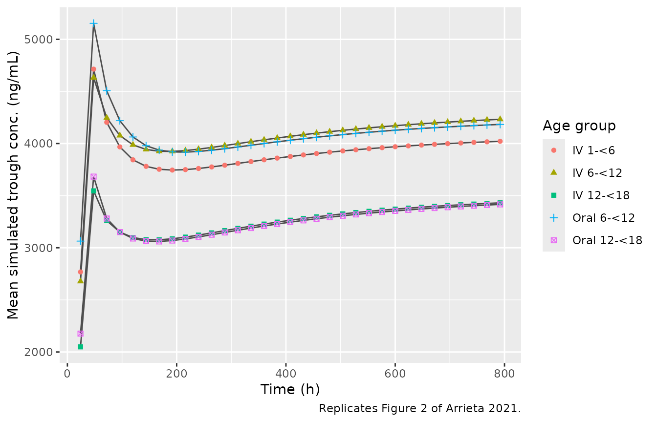
The maintainers digitised Figure 2 of the paper at two points: the 48-h trough after the loading phase (its peak) and the last plotted point (about 792 h, day 33). The table compares those values with the simulated mean troughs.
fig2_digitised <- tibble::tribble(
  ~cohort,       ~time,  ~paper_ngml,
  "IV 1-<6",      47.99,  4852,
  "IV 6-<12",     47.99,  5083,
  "IV 12-<18",    47.99,  3653,
  "Oral 6-<12",   47.99,  5187,
  "Oral 12-<18",  47.99,  3904,
  "IV 1-<6",     791.99,  3850,
  "IV 6-<12",    791.99,  4440,
  "IV 12-<18",   791.99,  3540,
  "Oral 6-<12",  791.99,  4350,
  "Oral 12-<18", 791.99,  3600
)
fig2_cmp <- troughs |>
  mutate(cohort = as.character(cohort)) |>
  inner_join(fig2_digitised, by = c("cohort", "time")) |>
  mutate(pct_diff = 100 * (mean_trough_ngml / paper_ngml - 1))
stopifnot(nrow(fig2_cmp) == 10L)

fig2_cmp |>
  select(cohort, time, paper_ngml, mean_trough_ngml, pct_diff) |>
  rename(
    "Cohort" = cohort,
    "Time (h)" = time,
    "Figure 2 (ng/mL, digitised)" = paper_ngml,
    "Simulated mean (ng/mL)" = mean_trough_ngml,
    "% diff" = pct_diff
  ) |>
knitr::kable(digits = 1, caption = "Mean trough after the loading phase (48 h) and near day 33 (792 h).")| Cohort | Time (h) | Figure 2 (ng/mL, digitised) | Simulated mean (ng/mL) | % diff |
|---|---|---|---|---|
| IV 1-<6 | 48 | 4852 | 4714.0 | -2.8 |
| IV 1-<6 | 792 | 3850 | 4021.5 | 4.5 |
| IV 6-<12 | 48 | 5083 | 4631.8 | -8.9 |
| IV 6-<12 | 792 | 4440 | 4232.6 | -4.7 |
| IV 12-<18 | 48 | 3653 | 3545.8 | -2.9 |
| IV 12-<18 | 792 | 3540 | 3431.0 | -3.1 |
| Oral 6-<12 | 48 | 5187 | 5153.5 | -0.6 |
| Oral 6-<12 | 792 | 4350 | 4183.5 | -3.8 |
| Oral 12-<18 | 48 | 3904 | 3682.7 | -5.7 |
| Oral 12-<18 | 792 | 3600 | 3416.0 | -5.1 |
stopifnot(
  # Structural: a wrong CL, dose conversion or allometric exponent shifts
  # every cohort by tens of percent. Observed: median about -4%, largest
  # about 9% (i.v. 6 to <12 at 48 h). A 200-subject mean at this IIV carries
  # about 4% sampling error, and the cohort weight distribution behind
  # Figure 2 is unpublished, hence the headroom.
  abs(median(fig2_cmp$pct_diff)) < 10,
  max(abs(fig2_cmp$pct_diff)) < 20
)
Figure 1 and Table 3: steady-state AUC and target attainment
At true steady state, the AUC over one dosing interval equals
F * dose / CL. The table checks the PKNCA AUC over the
day-33 interval against that identity for every simulated subject
(fdepot = 1 for i.v., 0.95 oral). The two sides share the
drawn parameters, so any gap is residual accumulation into the deep
compartment plus numerical error.
sim_nca <- sim |>
  filter(!is.na(Cc)) |>
  select(id, time, Cc, cohort)
sim_nca <- bind_rows(
  sim_nca,
  sim_nca |> distinct(id, cohort) |> mutate(time = 0, Cc = 0)
) |>
  distinct(id, cohort, time, .keep_all = TRUE) |>
  arrange(id, cohort, time)

conc_obj <- PKNCA::PKNCAconc(sim_nca, Cc ~ time | cohort + id)
dose_df <- events |>
  filter(evid == 1) |>
  select(id, time, amt, cohort)
dose_obj <- PKNCA::PKNCAdose(dose_df, amt ~ time | cohort + id)

intervals <- data.frame(
  start = c(143.99, 767.99),
  end = c(167.99, 791.99),
  cmax = TRUE,
  tmax = TRUE,
  auclast = TRUE
)
nca_res <- PKNCA::pk.nca(PKNCA::PKNCAdata(conc_obj, dose_obj, intervals = intervals))
nca_df <- as.data.frame(nca_res$result)

auc_ss <- nca_df |>
  filter(start == 767.99, PPTESTCD == "auclast") |>
  select(id, cohort, auc_ss = PPORRES) |>
  left_join(
    sim |>
      filter(time == max(ss_grid)) |>
      select(id, cl, dose_mg, route),
    by = "id"
  ) |>
  mutate(
    auc_closed = ifelse(route == "oral", 0.95, 1) * dose_mg / cl,
    pct_ss = 100 * (auc_ss / auc_closed - 1)
  )

stopifnot(
  # The simulated day-33 interval is essentially at steady state. Subjects
  # with a large deep volume (68% CV on V4) are still accumulating slightly,
  # so the tail is a little wider than the centre.
  abs(median(auc_ss$pct_ss)) < 2,
  quantile(abs(auc_ss$pct_ss), 0.9) < 5
)
summary(auc_ss$pct_ss)
#>      Min.   1st Qu.    Median      Mean   3rd Qu.      Max.
#> -62.13083  -0.45268  -0.11426  -1.51278  -0.04957   0.34525
fig1_digitised <- tibble::tribble(
  ~cohort,       ~paper_median,
  "IV 1-<6",     103,
  "IV 6-<12",    118,
  "IV 12-<18",    91,
  "Oral 6-<12",  108,
  "Oral 12-<18",  88
)

ggplot(auc_ss, aes(cohort, auc_ss, fill = cohort)) +
  geom_boxplot(outlier.shape = 1, show.legend = FALSE) +
  geom_hline(yintercept = c(60, 233), colour = c("blue", "green3")) +
  geom_point(
    data = fig1_digitised |> mutate(cohort = factor(cohort, levels = levels(auc_ss$cohort))),
    aes(cohort, paper_median), inherit.aes = FALSE, shape = 4, size = 4
  ) +
  labs(
    x = "Age group", y = "AUCss (ug*h/mL)",
    caption = "Replicates Figure 1 of Arrieta 2021 (pediatric boxes). X = digitised published median."
  )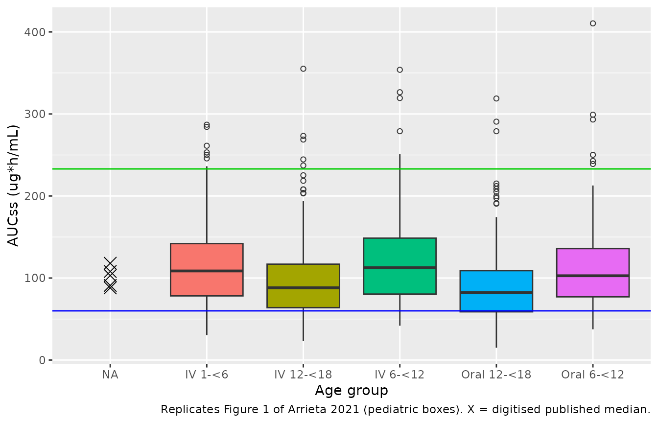
fig1_cmp <- auc_ss |>
  group_by(cohort) |>
  summarise(sim_median = median(auc_ss), .groups = "drop") |>
  mutate(cohort = as.character(cohort)) |>
  inner_join(fig1_digitised, by = "cohort") |>
  mutate(pct_diff = 100 * (sim_median / paper_median - 1))
fig1_cmp |>
  rename(
    "Cohort" = cohort,
    "Simulated median AUCss" = sim_median,
    "Figure 1 median (digitised)" = paper_median,
    "% diff" = pct_diff
  ) |>
knitr::kable(digits = 1, caption = "Median AUCss (ug*h/mL) by cohort.")| Cohort | Simulated median AUCss | Figure 1 median (digitised) | % diff |
|---|---|---|---|
| IV 1-<6 | 108.6 | 103 | 5.5 |
| IV 12-<18 | 88.2 | 91 | -3.1 |
| IV 6-<12 | 112.6 | 118 | -4.6 |
| Oral 12-<18 | 82.4 | 88 | -6.4 |
| Oral 6-<12 | 102.8 | 108 | -4.8 |
stopifnot(
  # Standard error of a 200-subject median at 45% CV is about 4%.
  abs(median(fig1_cmp$pct_diff)) < 10,
  max(abs(fig1_cmp$pct_diff)) < 20
)
Table 3 reports the percentage of simulated children below 60 and within 60 to 233 ugh/mL. Two estimates are shown for comparison. One uses the stochastic cohort above. The other is a semi-analytic value: with CL log-normal and AUCss = F dose / CL, the probability for each subject in the weight grid is a normal CDF on log CL, averaged over the grid. The semi-analytic value involves no random draws and is the one gated.
omega_cl <- sqrt(0.20394)
semi <- subjects |>
  mutate(
    auc_typ = ifelse(route == "oral", 0.95, 1) * dose_mg / (2.55 * (WT / 70)^0.75),
    p_below = pnorm((log(60) - log(auc_typ)) / omega_cl),
    p_within = pnorm((log(233) - log(auc_typ)) / omega_cl) - p_below
  ) |>
  group_by(cohort) |>
  summarise(semi_below = 100 * mean(p_below), semi_within = 100 * mean(p_within), .groups = "drop")

stoch <- auc_ss |>
  group_by(cohort) |>
  summarise(
    sim_below = 100 * mean(auc_ss < 60),
    sim_within = 100 * mean(auc_ss >= 60 & auc_ss <= 233),
    .groups = "drop"
  )

table3 <- tibble::tribble(
  ~cohort,       ~paper_below, ~paper_within,
  "IV 1-<6",       11.4,         85.7,
  "IV 6-<12",       7.2,         86.8,
  "IV 12-<18",     18.0,         80.2,
  "Oral 6-<12",     9.3,         87.1,
  "Oral 12-<18",   21.6,         76.5
)

t3 <- table3 |>
  inner_join(semi |> mutate(cohort = as.character(cohort)), by = "cohort") |>
  inner_join(stoch |> mutate(cohort = as.character(cohort)), by = "cohort")

t3 |>
  rename(
    "Cohort" = cohort,
    "Below 60, paper (%)" = paper_below,
    "Below 60, semi-analytic (%)" = semi_below,
    "Below 60, simulated (%)" = sim_below,
    "60-233, paper (%)" = paper_within,
    "60-233, semi-analytic (%)" = semi_within,
    "60-233, simulated (%)" = sim_within
  ) |>
  select(1, 2, 4, 6, 3, 5, 7) |>
knitr::kable(digits = 1, caption = "Replicates Table 3 of Arrieta 2021.")| Cohort | Below 60, paper (%) | Below 60, semi-analytic (%) | Below 60, simulated (%) | 60-233, paper (%) | 60-233, semi-analytic (%) | 60-233, simulated (%) |
|---|---|---|---|---|---|---|
| IV 1-<6 | 11.4 | 12.5 | 10.0 | 85.7 | 84.2 | 86.5 |
| IV 6-<12 | 7.2 | 9.3 | 11.0 | 86.8 | 85.4 | 86.0 |
| IV 12-<18 | 18.0 | 21.0 | 22.5 | 80.2 | 76.1 | 75.0 |
| Oral 6-<12 | 9.3 | 11.0 | 8.0 | 87.1 | 84.5 | 89.0 |
| Oral 12-<18 | 21.6 | 24.1 | 26.0 | 76.5 | 73.7 | 72.5 |
stopifnot(
  # Deterministic (no random draws). Observed gaps are at most about 4
  # percentage points and come from the unpublished simulated weight
  # distribution. A 10-fold IIV or a wrong allometric exponent moves these by
  # 10+ points.
  max(abs(t3$semi_below - t3$paper_below)) < 6,
  max(abs(t3$semi_within - t3$paper_within)) < 6
)
PKNCA validation against observed day-7 NCA
Table 2 of the paper reports noncompartmental Cmax, AUCtau and Tmax from the observed day-7 profiles. These come from 5 to 9 patients per cohort, whose weights differ from the virtual cohort above, so the comparison is descriptive. The day-7 interval here runs from the 144-h dose to the next dose.
published_day7 <- tibble::tribble(
  ~cohort,       ~cmax, ~auclast, ~tmax,
  "IV 1-<6",      7.31,  102.0,   1.08,
  "IV 6-<12",     6.97,   78.2,   1.08,
  "IV 12-<18",    5.65,   77.8,   1.07,
  "Oral 6-<12",   5.78,  121.0,   4.00,
  "Oral 12-<18",  5.43,   76.7,   3.98
)

day7 <- nca_df |>
  filter(start == 143.99) |>
  mutate(
    cohort = as.character(cohort),
    # report tmax relative to the day-7 dose
    PPORRES = ifelse(PPTESTCD == "tmax", PPORRES - (144 - 143.99), PPORRES)
  )

cmp <- nlmixr2lib::ncaComparisonTable(
  simulated = day7,
  reference = published_day7,
  by = "cohort",
  units = c(cmax = "ug/mL", auclast = "ug*h/mL", tmax = "h"),
  tolerance_pct = 20
)
knitr::kable(
  cmp,
  caption = "Day 7: simulated median vs. observed median NCA (Arrieta 2021 Table 2). * differs by >20%."
)| NCA parameter | cohort | Reference | Simulated | % diff |
|---|---|---|---|---|
| Cmax (ug/mL) | IV 1-<6 | 7.31 | 9.84 | +34.7%* |
| Cmax (ug/mL) | IV 6-<12 | 6.97 | 9.9 | +42.1%* |
| Cmax (ug/mL) | IV 12-<18 | 5.65 | 7.63 | +35.0%* |
| Cmax (ug/mL) | Oral 6-<12 | 5.78 | 4.58 | -20.8%* |
| Cmax (ug/mL) | Oral 12-<18 | 5.43 | 3.58 | -34.0%* |
| Tmax (h) | IV 1-<6 | 1.08 | 1 | -7.4% |
| Tmax (h) | IV 6-<12 | 1.08 | 1 | -7.4% |
| Tmax (h) | IV 12-<18 | 1.07 | 1 | -6.5% |
| Tmax (h) | Oral 6-<12 | 4 | 2.99 | -25.2%* |
| Tmax (h) | Oral 12-<18 | 3.98 | 2.99 | -24.9%* |
| AUClast (ug*h/mL) | IV 1-<6 | 102 | 107 | +4.6% |
| AUClast (ug*h/mL) | IV 6-<12 | 78.2 | 105 | +33.7%* |
| AUClast (ug*h/mL) | IV 12-<18 | 77.8 | 81.6 | +4.9% |
| AUClast (ug*h/mL) | Oral 6-<12 | 121 | 96.3 | -20.4%* |
| AUClast (ug*h/mL) | Oral 12-<18 | 76.7 | 77.5 | +1.0% |
Day-7 AUCtau agrees within 5% for three cohorts. It is 34% high for the i.v. 6 to <12 cohort and 20% low for the oral 6 to <12 cohort. Both simulated values fall inside the observed ranges (56.0-144.0 and 48.6-185.0 ug*h/mL). In Table 2 the i.v. 6 to <12 median (78.2) is below the i.v. 1 to <6 median (102), whereas the model, like the paper’s own Figure 1 simulation, puts the 6 to <12 cohort slightly higher. The oral 6 to <12 median (121) is the highest in Table 2, from 7 patients.
The largest discrepancy is Cmax, which is starred in every cohort. For the i.v. cohorts the simulated Cmax is taken at the exact end of the 1-h infusion. The rapid first distribution phase (Q3/V2 about 1.7 1/h) makes that value very sensitive to sampling time. The protocol sample was drawn within 5 min after the infusion ended, and the observed median Tmax was 1.07-1.08 h. The table below gives the simulated concentration at 1.08 h after the start of the infusion. It narrows the gap from 35-42% to about 20-27% but does not close it. The i.v. peak is therefore the part of the profile this model reproduces least well; AUC and trough exposure, which the paper used for dosing, are reproduced closely. The simulated oral peak is lower and earlier (about 3 h rather than 4 h) than observed, which is consistent with the single first-order Ka.
iv_peak <- sim |>
  filter(route == "iv", time == round(143.99 + 1.08, 2)) |>
  group_by(cohort) |>
  summarise(sim_c108 = median(Cc), .groups = "drop") |>
  mutate(cohort = as.character(cohort)) |>
  inner_join(published_day7 |> select(cohort, cmax), by = "cohort") |>
  mutate(pct_diff = 100 * (sim_c108 / cmax - 1))

iv_peak |>
  rename(
    "Cohort" = cohort,
    "Simulated median Cc at 1.08 h (ug/mL)" = sim_c108,
    "Observed median Cmax (ug/mL)" = cmax,
    "% diff" = pct_diff
  ) |>
knitr::kable(digits = 2, caption = "Day-7 i.v. peak at the protocol sampling time.")| Cohort | Simulated median Cc at 1.08 h (ug/mL) | Observed median Cmax (ug/mL) | % diff |
|---|---|---|---|
| IV 1-<6 | 8.76 | 7.31 | 19.82 |
| IV 6-<12 | 8.82 | 6.97 | 26.50 |
| IV 12-<18 | 6.87 | 5.65 | 21.62 |
Assumptions and deviations
- Zero-order input = the i.v. infusion. The paper describes “a 3-compartment model with combined zero-order and first-order input”. Table S2 lists no zero-order duration (D1) or lag time. The only reading consistent with the published estimates is that the i.v. doses are 1-h zero-order infusions and the oral doses are first-order absorption (Ka, F1), so the model encodes that.
-
Allometric exponents. The Methods give
P_pediatric = P_adults * (WT/70)^xbut never print x. No exponent appears among the estimates in Table S2, so the conventional fixed values were used: 0.75 on CL, Q3 and Q4, and 1 on V2, V3 and V4. The good agreement with Figure 1 and Table 3 supports this. The paper labels the equation as pediatric scaling. In this implementation the same (WT/70) scaling applies to adults too, which changes an adult near 70 kg only slightly. - IIV scale. Table S2 reports each IIV as a CV%. The printed SE and %RSE columns are consistent with omega^2 = (CV/100)^2 (CL, Q4, V4). The V3 row’s RSE (61%) matches neither reading and looks like a transcription slip in the table. No covariances are reported, so the omega matrix is diagonal.
-
Residual error. The table’s “sigma^2 = 40.86” sits
under the Variability (%) heading. Its SE (0.00934) and RSE (6%) show
that 40.86 is the SD in percent. Figure S2 is on log-concentration axes,
so the error model is log-transform-both-sides additive, encoded as
proportional in linear space (
propSd = 0.4086). - Dose units. Doses are in mg of isavuconazole. 372 mg isavuconazonium sulfate = 200 mg isavuconazole (Results, ‘ISAV exposure’), so 10 mg/kg of prodrug = 5.38 mg/kg of isavuconazole. Oral doses were not rounded to whole 74.5-mg capsules.
- Virtual cohort. The paper does not describe how weights were generated for its 1,000-subject simulations. Pooling the i.v. and oral patients of an age band (geometric mean of the two cohort medians, clamped to the pooled observed range) reproduced the Figure 1 medians better than cohort-specific weights did. With cohort-specific weights, the i.v. 12 to <18 median was 82 rather than 91 ug*h/mL. The maintenance phase starts 8 h after the last loading dose. The paper allowed the loading phase to end on day 2 or day 3 (Table S1 footnote).
-
Adult cohort. The adult phase 1 data (Townsend
2017) were part of the fit, but this paper reports no adult demographics
or adult simulations. The model’s
populationmetadata therefore describes the pediatric cohorts. - Errata. No correction notice for this article was found in Crossref as of 2026-09-28.