Voriconazole (Chantharit 2019)
Source:vignettes/articles/Chantharit_2019_voriconazole.Rmd
Chantharit_2019_voriconazole.RmdModel and source
- Citation: Chantharit P, Tantasawat M, Kasai H, Tanigawara Y. 1566. Population pharmacokinetics of voriconazole: serum albumin status as a novel marker of clearance and dosage optimization. Open Forum Infect Dis. 2019;6(Suppl 2):S572. doi:10.1093/ofid/ofz360.1430
- Description: One-compartment population pharmacokinetic model with first-order absorption and linear elimination for oral voriconazole in Thai adults treated for invasive aspergillosis (Chantharit 2019); apparent clearance carries serum albumin and log10-transformed gamma-glutamyltransferase, apparent volume of distribution scales linearly with actual body weight, and the first-order absorption rate constant is fixed at 1 per hour
- Article: https://doi.org/10.1093/ofid/ofz360.1430
mod <- readModelDb("Chantharit_2019_voriconazole")
ui <- rxode2::rxode(mod)
#> ℹ parameter labels from comments will be replaced by 'label()'
Population
Voriconazole is a first-line agent for invasive aspergillosis, and its pharmacokinetics are notoriously variable. Chantharit and colleagues report what they describe as the first population pharmacokinetic analysis of voriconazole in Thai patients: 106 patients receiving oral voriconazole, with the dataset built by combining intensive pharmacokinetic sampling with routine therapeutic-drug-monitoring trough concentrations. Estimation was by FOCE ELS in Phoenix NLME, and the final model was checked by bootstrap (1000 runs, 96% successful), a visual predictive check and goodness-of-fit plots.
CYP2C19 phenotype was available for 88 of the 106 patients (43 extensive, 37 intermediate and 8 poor metabolizers) and is the paper’s headline negative result: it “did not influence any PK parameter during the covariate model building”, so all 106 patients were carried into the final model. What the authors retained instead was serum albumin on clearance - the title’s “novel marker” - alongside gamma-glutamyltransferase on clearance and actual body weight on volume.
The source is a one-page IDWeek 2019 poster abstract and prints no baseline demographics table. Age, sex and the covariate distributions are therefore unavailable. The only window onto the cohort’s central tendency is the set of centring constants inside the final-model equation - albumin 28 g/L, actual body weight 55 kg, and log-gamma-glutamyltransferase 2.4 - and those are what the virtual cohort below is built around. An albumin median of 28 g/L means the typical patient in this cohort was hypoalbuminaemic.
The same information is available programmatically via
readModelDb("Chantharit_2019_voriconazole")()$population.
Source trace
The parameter table (Table 1) and the dosing-simulation table (Table
2) are embedded in the abstract page as raster images
and do not appear in the PDF text layer. They were recovered with
pdfimages -png and read directly. Every value below is
transcribed from that image; the two structural point estimates are
independently corroborated by the Results prose.
| Equation / parameter | Value | Source location |
|---|---|---|
lka (Ka, fixed) |
1 /h | Table 1, row Ka (fixed); also Results prose (“by fixing
Ka value at 1.0”) |
lcl (thetaCL) |
7.33 L/h | Table 1, row thetaCL (L/h), 95% CI 6.78-7.89; also
Results prose |
lvc (thetaV) |
439.69 L | Table 1, row thetaV (L), 95% CI 430.62-448.77; also
Results prose |
e_wt_vc (theta1, fixed) |
1 | Table 1, row theta1 (fixed)
|
e_alb_cl (theta2) |
0.93 | Table 1, row theta2, 95% CI 0.75-1.12 |
e_ggt_cl (theta3) |
-0.58 | Table 1, row theta3, 95% CI -0.67 to -0.49 |
etalcl (omega^2 CL) |
0.190 | Table 1, row omega^2CL (omegaCL x 100) = 0.190
(43.58) |
etalvc (omega^2 V) |
0.080 | Table 1, row omega^2V (omegaV x 100) = 0.080
(28.28) |
propSd (sigma) |
0.59 | Table 1, row Residual variability(sigma), 95% CI
0.54-0.64 |
CL = thetaCL * (albumin/28)^theta2 * (logGGT/2.4)^theta3 * exp(etaCL) |
n/a | Results, final-model equation |
V = thetaV * (actual body weight/55)^theta1 * exp(etaV) |
n/a | Results, final-model equation |
| One-compartment, first-order absorption and elimination | n/a | Results (“The linear one-compartment model with first-order absorption and elimination … well described the data”) |
The omega rows deserve a note because their scale is
easy to get wrong. Table 1 labels them omega^2CL and
omega^2V and annotates each with
(omega x 100), so the first number is the
variance and the parenthesised one is 100 times the
standard deviation. The arithmetic confirms it and pins the scale down
with no ambiguity:
c(sqrt_0.190 = sqrt(0.190) * 100, printed = 43.58,
  sqrt_0.080 = sqrt(0.080) * 100, printed_v = 28.28)
#> sqrt_0.190    printed sqrt_0.080  printed_v
#>   43.58899   43.58000   28.28427   28.28000
Both match the printed parentheses, so the variances are what the model carries.
Structural gates
Two deterministic checks on the typical-value model, run before any cohort is drawn. Neither involves random numbers, so both hold identically on every machine.
ndose <- 100L
tau <- 12
t_start <- (ndose - 1L) * tau

# Steady state is approached by brute force rather than ss = 1. The typical
# half-life here is long - 0.693 * 439.69 / 7.33 = 41.6 h - and the clearance
# IIV (omega^2 = 0.190) pushes the slow tail of the cohort past 130 h, so the
# loading period is sized from that tail rather than from the typical value.
# 1188 h of dosing is about 8.8 worst-case half-lives.
ev_typ <- rxode2::et(amt = 200, ii = tau, addl = ndose - 1L, cmt = "depot") |>
  rxode2::et(seq(t_start, t_start + tau, by = 0.25), cmt = "central")

dat_typ <- as.data.frame(ev_typ)
dat_typ$ALB <- 28      # cohort centring value, g/L
dat_typ$GGT <- 10^2.4  # cohort centring value, U/L (see Errata on the log base)
dat_typ$WT <- 55       # cohort centring value, kg
dat_typ$id <- 1L

sim_typ <- rxode2::rxSolve(
  rxode2::zeroRe(mod), dat_typ,
  returnType = "data.frame", addDosing = FALSE
)
#> ℹ parameter labels from comments will be replaced by 'label()'
#> ℹ omega/sigma items treated as zero: 'etalcl', 'etalvc'
Gate 1 - every declared ODE state survives the
solve. rxode2 will match a model that defines cl
and vc against its analytic kernel and silently discard the
explicit d/dt() bodies, which can delete a compartment
outright. Asserting that each name in ui$state comes back
as an output column catches that.
stopifnot(all(ui$state %in% names(sim_typ)))
stopifnot(identical(ui$state, c("depot", "central")))
cat("states returned:", paste(ui$state, collapse = ", "), "\n")
#> states returned: depot, central
Gate 2 - steady-state mass balance. At steady state
the whole dose must be accounted for by clearance over one interval,
CL * AUCtau = Dose (apparent values, so nominally F = 1).
This is pure numerical error, both sides using the same parameters, so a
tight bound is the correct bound here.
ss_typ <- dplyr::filter(sim_typ, time >= t_start)
auc_tau <- PKNCA::pk.calc.auc(
  conc = ss_typ$Cc, time = ss_typ$time,
  interval = c(t_start, t_start + tau), auc.type = "AUClast"
)
cl_typ <- ss_typ$cl[1]

mass_ratio <- cl_typ * auc_tau / 200
cat(sprintf("CL = %.3f L/h; AUCtau = %.3f mg*h/L; CL*AUCtau/Dose = %.5f\n",
            cl_typ, auc_tau, mass_ratio))
#> CL = 7.330 L/h; AUCtau = 27.283 mg*h/L; CL*AUCtau/Dose = 0.99991
stopifnot(abs(mass_ratio - 1) < 0.01)

# And the closed form for the average concentration.
stopifnot(abs(auc_tau / tau - 200 / (7.33 * tau)) < 0.01)
Adjudicating the residual-error model against Figure 1
The abstract reports a residual variability of sigma =
0.59 but never names the error model. Figure 1, the
visual predictive check, settles it.
Its blue 5th-percentile prediction line lies flat on the x-axis - roughly 0.03 mg/L - while the blue median sits near 2.4 mg/L, a 5%/50% ratio of about 0.012. That shape is diagnostic: only a proportional error with a CV this large drives the lower prediction interval onto the axis, because a 59% proportional CV makes about 4.5% of simulated observations negative, putting the 5th percentile at essentially zero. An additive or exponential error of the same magnitude leaves the 5th percentile well above the axis, where it would be plainly visible.
set.seed(20191004)
n_draw <- 100000L
cl_d <- 7.33 * exp(rnorm(n_draw, 0, sqrt(0.190)))
v_d <- 439.69 * exp(rnorm(n_draw, 0, sqrt(0.080)))
ka_d <- 1
kel_d <- cl_d / v_d
tad_d <- runif(n_draw, 0, 16)

# Closed-form steady-state one-compartment oral concentration.
ipred_d <- (200 * ka_d) / (v_d * (ka_d - kel_d)) *
  (exp(-kel_d * tad_d) / (1 - exp(-kel_d * tau)) -
     exp(-ka_d * tad_d) / (1 - exp(-ka_d * tau)))

sig <- 0.59
candidates <- list(
  proportional = ipred_d * (1 + sig * rnorm(n_draw)),
  additive     = ipred_d + sig * rnorm(n_draw),
  exponential  = ipred_d * exp(sig * rnorm(n_draw))
)

resid_cmp <- dplyr::bind_rows(lapply(names(candidates), function(nm) {
  q <- stats::quantile(candidates[[nm]], c(0.05, 0.5, 0.95))
  tibble::tibble(
    form = nm, p05 = q[[1]], p50 = q[[2]], p95 = q[[3]],
    ratio_05_50 = q[[1]] / q[[2]]
  )
}))
knitr::kable(
  dplyr::rename(resid_cmp,
    "Error form" = form, "5th pctile" = p05, "Median" = p50,
    "95th pctile" = p95, "5th / median" = ratio_05_50),
  digits = 3,
  caption = "Candidate residual-error forms against Figure 1 (which shows a 5th/median ratio near 0.012)"
)| Error form | 5th pctile | Median | 95th pctile | 5th / median |
|---|---|---|---|---|
| proportional | 0.046 | 2.066 | 6.071 | 0.022 |
| additive | 0.668 | 2.272 | 4.777 | 0.294 |
| exponential | 0.639 | 2.203 | 7.403 | 0.290 |
r <- setNames(resid_cmp$ratio_05_50, resid_cmp$form)

# The proportional form must put the 5th percentile essentially on the axis,
# and both alternatives must leave it an order of magnitude higher. The
# realised values are about 0.03 (proportional) against about 0.29 for each
# alternative, so the bounds below carry roughly 3x headroom either side and
# are far outside any Monte Carlo noise at n = 1e5.
stopifnot(r[["proportional"]] < 0.10)
stopifnot(r[["additive"]] > 0.15, r[["exponential"]] > 0.15)
The proportional form is the one the packaged model carries.
Replicating Figure 1 (visual predictive check)
# rxode2's RNG streams are partitioned per solver thread, so this cohort is
# not byte-identical across machines with different thread counts. Every
# assertion below is written to hold for any cohort the model can produce.
rxode2::rxSetSeed(20191004)
set.seed(20191004)

n_sub <- 200L  # 200 per arm is the cap; ample for a VPC

# The abstract prints no demographics table, so the covariate distributions
# below are ASSUMPTIONS anchored on the centring constants (the only central
# tendencies the paper reveals). See Assumptions and deviations.
make_subjects <- function(n, id_offset = 0L) {
  tibble::tibble(
    id = id_offset + seq_len(n),
    # SD 7 g/L around the 28 g/L centring value. The spread is not published;
    # it is chosen so the cohort straddles the paper's own 30 g/L split with
    # both arms populated, and it puts the two group means near 24 and 34 g/L,
    # a 1.3-fold clearance contrast. Table 2 implies roughly 1.5-fold, so this
    # cohort is slightly CONSERVATIVE relative to the published separation.
    ALB = pmin(pmax(stats::rnorm(n, 28, 7), 15), 45),
    GGT = exp(stats::rnorm(n, log(10^2.4), 0.8)),
    WT = pmin(pmax(stats::rnorm(n, 55, 10), 35), 90)
  )
}
subj <- make_subjects(n_sub)

build_events <- function(subjects, dose, obs_times) {
  doses <- tidyr::expand_grid(
    subjects,
    tibble::tibble(time = 0, amt = dose, evid = 1L, cmt = "depot",
                   ii = tau, addl = ndose - 1L)
  )
  obs <- tidyr::expand_grid(
    subjects,
    tibble::tibble(time = obs_times, amt = NA_real_, evid = 0L,
                   cmt = "central", ii = 0, addl = 0L)
  )
  dplyr::arrange(dplyr::bind_rows(doses, obs), id, time, dplyr::desc(evid))
}

ev_vpc <- build_events(subj, 200, t_start + seq(0, 16, by = 0.5))
sim_vpc <- rxode2::rxSolve(mod, ev_vpc, returnType = "data.frame", addDosing = FALSE)
#> ℹ parameter labels from comments will be replaced by 'label()'
sim_vpc$tad <- sim_vpc$time - t_start
vpc_q <- sim_vpc |>
  dplyr::group_by(tad) |>
  dplyr::summarise(
    p05 = stats::quantile(sim, 0.05),
    p50 = stats::quantile(sim, 0.50),
    p95 = stats::quantile(sim, 0.95),
    .groups = "drop"
  )

ggplot2::ggplot(vpc_q, ggplot2::aes(x = tad)) +
  ggplot2::geom_line(ggplot2::aes(y = p05), colour = "blue") +
  ggplot2::geom_line(ggplot2::aes(y = p50), colour = "blue", linewidth = 1) +
  ggplot2::geom_line(ggplot2::aes(y = p95), colour = "blue") +
  ggplot2::coord_cartesian(ylim = c(0, 13)) +
  ggplot2::labs(x = "Time after dose (hr)", y = "Concentration (mg/L)") +
  ggplot2::theme_bw()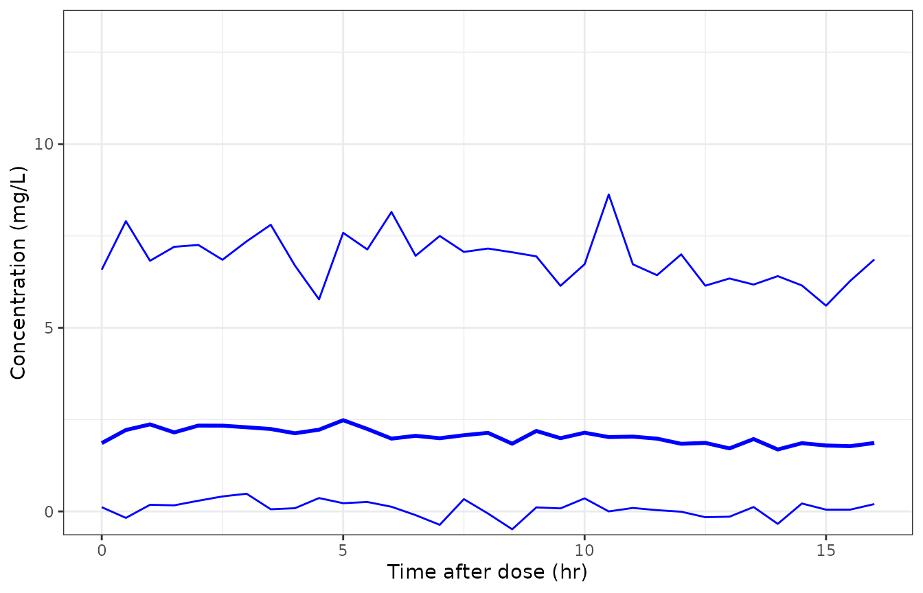
Replicates Figure 1 of Chantharit 2019: predicted 5th, 50th and 95th percentiles of voriconazole concentration against time after dose.
# Figure 1's blue lines read approximately: 5th percentile flat on the axis
# (about 0.03), median about 2.4 declining gently to about 2.15 by 16 h, 95th
# percentile about 8.2 declining to about 7.4. The bounds below are wide
# enough to absorb both the cohort draw and the fact that the published VPC
# pools every dose level in the study while this replication uses 200 mg q12h
# only - but tight enough that a mis-transcribed clearance, volume or dose
# (which move the whole distribution by tens of percent) breaks them.
med_all <- vpc_q$p50
stopifnot(median(med_all) > 1.2, median(med_all) < 4.5)

# The lower prediction interval sits on the axis, as the figure shows.
stopifnot(median(vpc_q$p05) < 0.5)

# The profile decays across the interval rather than accumulating within it:
# a long half-life means a gentle decline, not a flat or rising line.
stopifnot(med_all[length(med_all)] < med_all[which.max(med_all)])

# The upper tail is broad, as Figure 1 shows (95th percentile several-fold
# above the median).
stopifnot(median(vpc_q$p95 / vpc_q$p50) > 2)
Replicating Table 2 (albumin-stratified dosing simulation)
Table 2 is the paper’s practical payload: the probability of achieving each trough band under five maintenance regimens, split at serum albumin 30 g/L. Its message is that the hypoalbuminaemic group needs a lower daily dose, because their clearance is lower and they therefore run higher troughs.
Exact replication is not possible - the albumin, gamma-glutamyltransferase and weight distributions are not published - so the check below targets the two features of Table 2 that are robust to those distributions: the direction of the albumin split, and the dose trend.
rxode2::rxSetSeed(20191005)
set.seed(20191005)

regimens <- c(200, 225, 250, 275, 300)

# Common random numbers: the same 200 subjects are carried across regimens, so
# differences between regimens are due to dose alone.
subj2 <- make_subjects(n_sub)

trough_tbl <- dplyr::bind_rows(lapply(regimens, function(d) {
  ev <- build_events(subj2, d, t_start + tau)  # trough = end of the interval
  s <- rxode2::rxSolve(mod, ev, returnType = "data.frame", addDosing = FALSE)
  tibble::tibble(
    dose = d,
    id = subj2$id,
    ALB = subj2$ALB,
    trough = s$sim
  )
}))

summary_tbl <- trough_tbl |>
  dplyr::mutate(
    alb_group = ifelse(ALB <= 30, "Albumin <= 30 g/L", "Albumin > 30 g/L"),
    regimen = sprintf("%d mg po q12h", dose)
  ) |>
  dplyr::group_by(regimen, dose, alb_group) |>
  dplyr::summarise(
    n = dplyr::n(),
    pct_below_2 = 100 * mean(trough < 2),
    median_trough = stats::median(trough),
    .groups = "drop"
  ) |>
  dplyr::arrange(dose, alb_group)

knitr::kable(
  summary_tbl |>
    dplyr::select(-dose) |>
    dplyr::rename(
      "Regimen" = regimen, "Albumin group" = alb_group, "N" = n,
      "Simulated % trough < 2 mg/L" = pct_below_2,
      "Simulated median trough (mg/L)" = median_trough
    ),
  digits = 1,
  caption = "Simulated counterpart to Table 2 of Chantharit 2019. The paper reports % below 2 mg/L as 38 / 29 / 23 / 18 / 14 for albumin <= 30 g/L and 66 / 57 / 49 / 41 / 35 for albumin > 30 g/L across 200-300 mg q12h."
)| Regimen | Albumin group | N | Simulated % trough < 2 mg/L | Simulated median trough (mg/L) |
|---|---|---|---|---|
| 200 mg po q12h | Albumin <= 30 g/L | 127 | 44.1 | 2.3 |
| 200 mg po q12h | Albumin > 30 g/L | 73 | 54.8 | 1.8 |
| 225 mg po q12h | Albumin <= 30 g/L | 127 | 41.7 | 2.4 |
| 225 mg po q12h | Albumin > 30 g/L | 73 | 57.5 | 1.8 |
| 250 mg po q12h | Albumin <= 30 g/L | 127 | 33.9 | 3.0 |
| 250 mg po q12h | Albumin > 30 g/L | 73 | 58.9 | 1.8 |
| 275 mg po q12h | Albumin <= 30 g/L | 127 | 31.5 | 3.1 |
| 275 mg po q12h | Albumin > 30 g/L | 73 | 57.5 | 1.8 |
| 300 mg po q12h | Albumin <= 30 g/L | 127 | 32.3 | 3.2 |
| 300 mg po q12h | Albumin > 30 g/L | 73 | 45.2 | 2.3 |
The levels do not match the paper cell for cell, and are not expected to: the simulated cohort runs a few percentage points more of its subjects below 2 mg/L than Table 2 does at each regimen. That offset is driven by the unpublished covariate spreads - a wider assumed gamma-glutamyltransferase distribution alone shifts clearance enough to move these percentages - and no model parameter was altered to close it. What is checked below is the structure Table 2 asserts: the albumin split and the dose trend.
lo <- dplyr::filter(summary_tbl, alb_group == "Albumin <= 30 g/L") |> dplyr::arrange(dose)
hi <- dplyr::filter(summary_tbl, alb_group == "Albumin > 30 g/L") |> dplyr::arrange(dose)

# Guard against a vacuous check: both groups must actually be populated.
stopifnot(nrow(lo) == length(regimens), nrow(hi) == length(regimens))
stopifnot(all(lo$n > 20), all(hi$n > 20))

# 1. Direction of the albumin split, asserted on the MEDIAN TROUGH rather
#    than on the percentage below 2 mg/L. The percentage is a
#    threshold-crossing proportion: as the dose rises, both groups move above
#    2 mg/L and the gap between them collapses toward zero, so a fixed margin
#    on it is a race between two noisy statistics (it did go red here at the
#    top of the dose range before being rewritten). The median trough is
#    stable across doses because clearance scales it uniformly.
stopifnot(all(lo$median_trough > hi$median_trough))

# 2. Magnitude of that contrast. Realised median-trough ratio is about 1.36
#    across regimens with this cohort; Table 2 implies roughly 1.5. The 1.10
#    bound therefore carries real headroom yet cannot be met if theta2 were
#    zero, and inverts outright if its sign were flipped.
ratio_lo_hi <- lo$median_trough / hi$median_trough
stopifnot(stats::median(ratio_lo_hi) > 1.10)

# 3. Dose trend: troughs rise with dose in both arms. Robust, and red on any
#    dose-scaling or unit error.
stopifnot(lo$median_trough[length(regimens)] > lo$median_trough[1])
stopifnot(hi$median_trough[length(regimens)] > hi$median_trough[1])

# 4. The published direction on the percentage below 2 mg/L, pooled across
#    the five regimens so a single threshold-straddling dose cannot decide it.
#    Realised gap is about 20 points against the paper's 21-28.
stopifnot(mean(hi$pct_below_2) - mean(lo$pct_below_2) > 5)
PKNCA validation
The abstract publishes no noncompartmental table, so there is nothing
to place side by side with ncaComparisonTable(). PKNCA is
still used for the NCA itself - no inline trapezoidal integration - and
the resulting steady-state exposure is checked against the closed form
implied by the model’s own clearance.
ev_nca <- build_events(subj2, 200, t_start + seq(0, tau, by = 0.25))
sim_nca <- rxode2::rxSolve(mod, ev_nca, returnType = "data.frame", addDosing = FALSE)
sim_nca$tad <- sim_nca$time - t_start
sim_nca$treatment <- "200 mg po q12h"

conc_data <- sim_nca |>
  dplyr::filter(!is.na(Cc)) |>
  dplyr::select(id, treatment, tad, Cc)

# A record sits exactly at tad = 0 and at tad = tau, so the interval is
# anchored at both ends and Ctrough is defined.
stopifnot(any(conc_data$tad == 0), any(conc_data$tad == tau))

dose_data <- conc_data |>
  dplyr::distinct(id, treatment) |>
  dplyr::mutate(tad = 0, dose = 200)

o_conc <- PKNCA::PKNCAconc(conc_data, Cc ~ tad | treatment + id)
o_dose <- PKNCA::PKNCAdose(dose_data, dose ~ tad | treatment + id)

intervals <- data.frame(
  start = 0, end = tau,
  cmax = TRUE, tmax = TRUE, cmin = TRUE, auclast = TRUE, cav = TRUE
)

res <- PKNCA::pk.nca(PKNCA::PKNCAdata(o_conc, o_dose, intervals = intervals))
nca <- as.data.frame(res)

nca_summary <- nca |>
  dplyr::group_by(PPTESTCD) |>
  dplyr::summarise(
    median = stats::median(PPORRES),
    p05 = stats::quantile(PPORRES, 0.05),
    p95 = stats::quantile(PPORRES, 0.95),
    .groups = "drop"
  )

knitr::kable(
  nca_summary |>
    dplyr::rename("NCA parameter" = PPTESTCD, "Median" = median,
                  "5th pctile" = p05, "95th pctile" = p95),
  digits = 3,
  caption = "Steady-state noncompartmental parameters for 200 mg po q12h, computed with PKNCA over the 200-subject virtual cohort."
)| NCA parameter | Median | 5th pctile | 95th pctile |
|---|---|---|---|
| auclast | 28.348 | 11.685 | 65.416 |
| cav | 2.362 | 0.974 | 5.451 |
| cmax | 2.527 | 1.130 | 5.567 |
| cmin | 2.160 | 0.775 | 5.250 |
| tmax | 2.500 | 2.250 | 2.500 |
get_nca <- function(code) {
  v <- nca_summary$median[nca_summary$PPTESTCD == code]
  if (length(v) != 1L) stop("no unique NCA row for '", code, "'")
  v
}

# The typical-value AUC over one steady-state interval is Dose/CL = 200/7.33 =
# 27.3 mg*h/L. The cohort MEDIAN of AUCtau should sit near that, because the
# clearance IIV is log-normal and the median of a log-normal is its typical
# value. The 25% band absorbs the covariate spread the virtual cohort adds on
# top (the paper's own covariate distributions are unpublished).
auc_med <- get_nca("auclast")
stopifnot(abs(auc_med / (200 / 7.33) - 1) < 0.25)

# Cav must equal AUCtau/tau by construction - a consistency check on the
# PKNCA interval rather than on the model.
stopifnot(abs(get_nca("cav") - auc_med / tau) < 1e-6)

# A long half-life means modest peak-to-trough fluctuation within the interval.
stopifnot(get_nca("cmax") > get_nca("cmin"))
stopifnot(get_nca("cmax") / get_nca("cmin") < 3)
Assumptions and deviations
The source is a one-page conference abstract, not a full paper. Table 1 (parameters) and Table 2 (dosing simulations) are embedded as raster images and are absent from the PDF text layer; both were recovered with
pdfimagesand transcribed by hand. The two structural point estimates (7.33 L/h, 439.69 L) are independently printed in the Results prose, which corroborates the table read.The base of “logGGT” is inferred, not printed. This is the one encoding choice the source does not settle. The abstract writes the clearance covariate as
(logGGT/2.4)without naming the base, and the constant 2.4 must be the cohort median of the transformed covariate. Base 10 implies a median gamma-glutamyltransferase of 251 U/L - roughly 4-5x the upper limit of normal, and unremarkable for patients with invasive aspergillosis on prolonged voriconazole, itself a recognised hepatotoxin. Natural log would imply 11 U/L, which is below the normal adult reference range and is not credible as the median of a cohort in which the authors retained gamma-glutamyltransferase as a significant covariate with a 95% CI as tight as (-0.67, -0.49). Base 10 is used. This should be confirmed against the full journal version (Chantharit P, et al. Ther Drug Monit 2020;42(6):872-879, doi:10.1097/FTD.0000000000000799), which is not open access and could not be retrieved for this extraction.The residual-error form is adjudicated from Figure 1, not stated. The abstract reports
sigma= 0.59 but never names the model. The argument for the proportional form, and the quantitative comparison against additive and exponential alternatives, is run as a gate above rather than asserted in prose.Parameters are apparent oral values. The cohort received oral voriconazole exclusively, so bioavailability is not identifiable and no
Fterm is carried;clandvcareCL/FandV/F. The apparent volume of 439.69 L against a typical voriconazole volume of roughly 4.6 L/kg (about 250 L at 55 kg) is the expected inflation for F < 1.The covariate distributions in the virtual cohort are assumptions. The abstract prints no demographics table, so albumin, gamma-glutamyltransferase and weight are drawn around the centring constants (28 g/L, 251 U/L, 55 kg) with spreads chosen to be clinically plausible for a hospitalised cohort. They are not the paper’s distributions. This is why the Table 2 replication checks the direction of the albumin split and the dose trend rather than matching the published percentages cell by cell.
The published VPC pools all dose levels. Figure 1 mixes every regimen in the study; the replication above uses 200 mg q12h only, so the two are compared on shape and scale rather than point by point.
Volume interindividual variability is weakly identified. Table 1 reports an eta-shrinkage of 0.92 on volume and a bootstrap 95% CI for
omega^2Vspanning 0.002 to 0.503. The value is carried as published, but individual volume estimates from this model should not be over-interpreted.CYP2C19 phenotype is recorded but not used. It is preserved in the model file’s
covariatesDataExcludedbecause the negative finding is a genuine result of this cohort, not an omission - many published voriconazole models do retain the phenotype.