Linezolid (Abdelgawad 2024)
Source:vignettes/articles/Abdelgawad_2024_linezolid.Rmd
Abdelgawad_2024_linezolid.RmdModel and source
- Citation: Abdelgawad N, Wasserman S, Abdelwahab MT, Davis A, Stek C, Wiesner L, Black J, Meintjes G, Wilkinson RJ, Denti P (2024). Linezolid population pharmacokinetic model in plasma and cerebrospinal fluid among patients with tuberculosis meningitis. J Infect Dis 229(4):1200-1208. doi:10.1093/infdis/jiad413
- Description: One-compartment population PK model for oral linezolid in plasma and lumbar cerebrospinal fluid (CSF) in adults with HIV-associated tuberculous meningitis receiving high-dose rifampicin (35 mg/kg) co-treatment (LASER-TBM PK substudy, Abdelgawad 2024). Absorption is a Savic transit chain (mean transit time 0.211 h, estimated chain length 5.68) feeding a first-order depot (ka 1.21 1/h); elimination from the central compartment is saturable Michaelis-Menten with maximal clearance 7.25 L/h and Michaelis-Menten constant 27.2 mg/L, so Vmax = CLmax * km = 197 mg/h. CLmax and central volume (40.8 L) are allometrically scaled on fat-free mass with a 45 kg reference and fixed 0.75 / 1 exponents (FFM beat total body weight by dOFV -30 vs -7.7). CSF is a Sheiner-style effect compartment holding a concentration, equilibrating with plasma at 0.198 1/h (equilibration half-life 3.5 h) toward a pseudo-partition coefficient PPC; PPC rises linearly with CSF total protein and plateaus at PPCmax = 0.365 once CSF protein reaches an estimated 1.18 g/L breakpoint (a broken-stick whose intercept and amplitude were fixed to 0 and 1, so the slope 0.847 = 1/1.18 is fully determined by the breakpoint). Random effects are between-subject variability on CLmax (9.60%), between-visit variability on CLmax across the day-3 and day-28 PK visits (20.3%), and five-occasion between-occasion variability on ka (87.9%) and mean transit time (110%); all reported percentages are the omega standard deviation on the log scale. Residual error is combined proportional plus additive, separately for plasma (21.5%, 0.173 mg/L) and CSF (91.5%, 0.02 mg/L).
- Article: https://doi.org/10.1093/infdis/jiad413
- Supplement (assay methods, model-comparison table, figures S1-S4,
and the full NONMEM control file): supplementary data to the same DOI,
distributed by Oxford University Press as
jiad413_supplementary_data.zip.
Linezolid is being evaluated as part of intensified antibiotic regimens for tuberculous meningitis (TBM), where the drug must cross the blood-brain and blood-CSF barriers to reach the site of disease. This model is the first description of linezolid pharmacokinetics in plasma and lumbar cerebrospinal fluid in adults with TBM, and it was fitted to data collected while participants were also receiving high-dose (35 mg/kg) rifampicin – a potent enzyme inducer whose effect on linezolid exposure was a primary question of the analysis.
Population
The model was fitted to the pharmacokinetic substudy of LASER-TBM (ClinicalTrials.gov NCT03927313), a phase IIb open-label trial in adults with HIV-associated tuberculous meningitis enrolled at four public hospitals in Cape Town and Gqeberha, South Africa. Thirty participants underwent PK sampling on day 3 and 17 on day 28, contributing 247 plasma observations (6 below the limit of quantification, 2.43%) and 28 lumbar CSF observations (7 BLQ, 25%).
Baseline characteristics are Abdelgawad 2024 Table 1: median age 40 years (range 27-56), median weight 58 kg (range 30-96), median fat-free mass 45 kg (range 30-59), 60% male, median CD4 count 137 cells/mm3 (range 2-890). Median CSF total protein fell from 1.46 g/L (range 0.310-54.7) at the day-3 visit to 0.750 g/L (range 0.220-2.19) at day 28. Linezolid was given as 1200 mg orally once daily for 28 days and then reduced to 600 mg once daily; all participants also received rifampicin, isoniazid, pyrazinamide, ethambutol, and adjunctive dexamethasone.
The same information is available programmatically via the model’s
population metadata
(readModelDb("Abdelgawad_2024_linezolid")()$population).
Source trace
The per-parameter origin is recorded as an in-file comment next to
each ini() entry in
inst/modeldb/specificDrugs/Abdelgawad_2024_linezolid.R. The
table below collects them in one place for review. Final estimates come
from Abdelgawad 2024 Table 2; the supplementary NONMEM control file is
cited where it disambiguates the structure or the reporting scale.
| Equation / parameter | Value | Source location |
|---|---|---|
lvmax |
log(7.25 * 27.2) = log(197.2 mg/h) | Table 2 CLmax 7.25 L/h and km 27.2 mg/L; control file
$PK VMAX = CLMAX*KM
|
lkm |
log(27.2 mg/L) | Table 2 km 27.2 (16.0-46.4), RSE 29.1% |
lvc |
log(40.8 L) | Table 2 V 40.8 (37.9-43.6), RSE 3.65% |
lka |
log(1.21 1/h) | Table 2 ka 1.21 (.831-1.76), RSE 19.6% |
lmtt |
log(0.211 h) | Table 2 MTT 0.211 (.112-.342), RSE 28.6% |
lntr |
log(5.68) | Table 2 NN 5.68 (2.36-11.8), RSE 43.5% |
lfdepot |
fixed(log(1)) | Table 2 F 1 fixed; control file $THETA 5 FIX
|
lke0 |
log(0.198 1/h) | Table 2 k plasma-CSF 0.198 (.0849-.340), RSE 33.7% |
lppc |
log(0.365) | Table 2 PPCmax 0.365 (.238-.566), RSE 23.2% |
e_csftpro_ppc |
1.18 g/L | Table 2 CSF protein max 1.18 (.730-1.90), RSE 24.4% |
e_ffm_vmax |
fixed(0.75) | Results, PK Modeling; control file $PK
ALLMCL_FFM = (FFM/45)**0.75
|
e_ffm_vc |
fixed(1) | Results, PK Modeling; control file $PK
ALLMV_FFM = (FFM/45)
|
etalvmax |
0.009216 = 0.0960^2 | Table 2 BSV in CLmax 9.60% (3.44-13.9) |
etabvv_vmax_1, _2
|
0.041209 = 0.203^2 | Table 2 BVV in CLmax 20.3% (15.3-26.9); control file
$OMEGA BLOCK(1) 0.0411842 + SAME
|
etaiov_ka_1 .. _5
|
0.772641 = 0.879^2 | Table 2 BOV in ka 87.9% (66.4-110); control file
$OMEGA BLOCK(1) 0.772478 + 4x SAME
|
etaiov_mtt_1 .. _5
|
1.21 = 1.10^2 | Table 2 BOV in MTT 110% (75.8-144); control file
$OMEGA BLOCK(1) 1.19782 + 4x SAME
|
propSd |
0.215 | Table 2 Plasma proportional error 21.5% (18.8-24.7) |
addSd |
0.173 mg/L | Table 2 Plasma additive error 0.173 (.0379-.355) |
propSd_Ccsf |
0.915 | Table 2 CSF proportional error 91.5% (63.3-151) |
addSd_Ccsf |
fixed(0.02) mg/L | Table 2 CSF additive error 0.02 fixed; footnote c |
d/dt(depot) = transit(ntr, mtt, fdepot) - ka * depot,
f(depot) = 0
|
n/a | Control file $DES
DADT(1) = TRANSIT - KA*A(1) with the Savic gamma-density
TRANSIT; $PK F1 = 0,
KTR = (NN+1)/MTT
|
d/dt(central) = ka * depot - vmax * Cc / (km + Cc) |
n/a | Control file $DES
DADT(2) = KA*A(1) - ((VMAX/(KM+C2))/V)*A(2); Figure 1 |
d/dt(csf) = ke0 * (ppc * Cc - csf) |
n/a | Control file $DES
DADT(3) = KE0*(PPC*C2 - A(3)); Figure 1 |
ppc = PPCmax * min(CSF_TPRO / 1.18, 1) |
n/a | Control file $PK
SLP/COV_EFF/TVPPC block; Table 2
footnote e and Figure 2 (see Errata) |
Structural checks
Three relationships in the paper are pure arithmetic on the packaged parameters, so they can be checked exactly rather than graphically.
mod <- readModelDb("Abdelgawad_2024_linezolid")
th <- rxode2::rxode(mod)$theta
#> ℹ parameter labels from comments will be replaced by 'label()'
#> Warning: some etas defaulted to non-mu referenced, possible parsing error: etabvv_vmax_1, etabvv_vmax_2, etaiov_ka_1, etaiov_ka_2, etaiov_ka_3, etaiov_ka_4, etaiov_ka_5, etaiov_mtt_1, etaiov_mtt_2, etaiov_mtt_3, etaiov_mtt_4, etaiov_mtt_5
#> as a work-around try putting the mu-referenced expression on a simple line

structural <- tibble::tibble(
  Quantity = c(
    "Maximal clearance CLmax = Vmax / km (L/h)",
    "Plasma-CSF equilibration half-life = log(2) / ke0 (h)",
    "Broken-stick slope = PPCmax / breakpoint, per g/L",
    "Rise in PPC per 0.1 mg/mL of CSF protein (percentage points)",
    "PPC at the paper's typical CSF protein of 0.995 g/L"
  ),
  Model = c(
    exp(th[["lvmax"]]) / exp(th[["lkm"]]),
    log(2) / exp(th[["lke0"]]),
    exp(th[["lppc"]]) / th[["e_csftpro_ppc"]],
    100 * exp(th[["lppc"]]) / th[["e_csftpro_ppc"]] * 0.1,
    exp(th[["lppc"]]) * min(0.995 / th[["e_csftpro_ppc"]], 1)
  ),
  Published = c(7.25, 3.5, 0.847 * 0.365, 3, 0.31),
  `Source` = c(
    "Table 2 CLmax",
    "Table 2 footnote d",
    "Table 2 footnote e (slope 0.847, scaled by PPCmax)",
    "Results, PK Modeling ('an increase of 3% in PPC')",
    "Discussion ('on average ~30% of plasma exposure')"
  )
)

knitr::kable(structural, digits = 4,
caption = "Exact structural relationships versus the published values.")| Quantity | Model | Published | Source |
|---|---|---|---|
| Maximal clearance CLmax = Vmax / km (L/h) | 7.2500 | 7.2500 | Table 2 CLmax |
| Plasma-CSF equilibration half-life = log(2) / ke0 (h) | 3.5007 | 3.5000 | Table 2 footnote d |
| Broken-stick slope = PPCmax / breakpoint, per g/L | 0.3093 | 0.3092 | Table 2 footnote e (slope 0.847, scaled by PPCmax) |
| Rise in PPC per 0.1 mg/mL of CSF protein (percentage points) | 3.0932 | 3.0000 | Results, PK Modeling (‘an increase of 3% in PPC’) |
| PPC at the paper’s typical CSF protein of 0.995 g/L | 0.3078 | 0.3100 | Discussion (‘on average ~30% of plasma exposure’) |
The equilibration half-life reproduces the published 3.5 h to four
significant figures, and the broken-stick slope reproduces Table 2
footnote e’s 0.847 (which the footnote reports before multiplication by
PPCmax).
Virtual cohort
Original observed data are not publicly available. The simulations below use the typical participant the paper itself specifies for its Monte Carlo simulations (Methods, Simulations): a fat-free mass of 45 kg and a CSF total protein of 0.995 g/L, dosed to steady state with 600 or 1200 mg once daily. Two hundred participants per dose arm carry the published random effects.
set.seed(20240401)

tau <- 24        # dosing interval, h
n_dose <- 8      # doses to steady state (linezolid t1/2 is a few hours)
t_end <- tau * n_dose
n_per_arm <- 200 # cap: never more than 200 participants per arm

make_arm <- function(dose, id_offset) {
  ids <- id_offset + seq_len(n_per_arm)
  dosing <- tidyr::expand_grid(
    id = ids,
    time = seq(0, tau * (n_dose - 1), by = tau)
  ) |>
    dplyr::mutate(amt = dose, evid = 1L, cmt = "depot")
  # Observations are written on the endpoint name "Cc". This model declares two
  # endpoints (Cc and Ccsf), so rxode2 assigns each an endpoint slot after the
  # ODE states; naming one endpoint maps the row unambiguously and rxSolve
  # returns BOTH observables as columns. Using an ODE state name here instead
  # fails with "'dvid'->'cmt' on observation record".
  obs <- tidyr::expand_grid(
    id = ids,
    time = seq(0, t_end, by = 0.25)
  ) |>
    dplyr::mutate(amt = NA_real_, evid = 0L, cmt = "Cc")
  dplyr::bind_rows(dosing, obs) |>
    dplyr::mutate(
      FFM = 45,        # cohort median fat-free mass, Table 1
      CSF_TPRO = 0.995, # typical CSF total protein, Methods (Simulations)
      OCC = 1,
      treatment = paste(dose, "mg")
    ) |>
    dplyr::arrange(id, time, dplyr::desc(evid))
}

events <- dplyr::bind_rows(
  make_arm(1200, id_offset = 0L),
  make_arm(600, id_offset = 1000L)
)
stopifnot(!anyDuplicated(unique(events[, c("id", "time", "evid")])))
Simulation
# useLinCmt = FALSE: rxode2's automatic ODE-to-linCmt conversion corrupts the
# endpoint mapping for two-output models on [central, csf].
sim <- rxode2::rxSolve(
  mod, events = events,
  keep = c("treatment", "FFM", "CSF_TPRO"),
  useLinCmt = FALSE
) |>
  as.data.frame()
#> ℹ parameter labels from comments will be replaced by 'label()'
#> Warning: some etas defaulted to non-mu referenced, possible parsing error: etabvv_vmax_1, etabvv_vmax_2, etaiov_ka_1, etaiov_ka_2, etaiov_ka_3, etaiov_ka_4, etaiov_ka_5, etaiov_mtt_1, etaiov_mtt_2, etaiov_mtt_3, etaiov_mtt_4, etaiov_mtt_5
#> as a work-around try putting the mu-referenced expression on a simple line

mod_typical <- rxode2::zeroRe(mod)
#> ℹ parameter labels from comments will be replaced by 'label()'
#> Warning: some etas defaulted to non-mu referenced, possible parsing error: etabvv_vmax_1, etabvv_vmax_2, etaiov_ka_1, etaiov_ka_2, etaiov_ka_3, etaiov_ka_4, etaiov_ka_5, etaiov_mtt_1, etaiov_mtt_2, etaiov_mtt_3, etaiov_mtt_4, etaiov_mtt_5
#> as a work-around try putting the mu-referenced expression on a simple line
#> Warning: some etas defaulted to non-mu referenced, possible parsing error: etabvv_vmax_1, etabvv_vmax_2, etaiov_ka_1, etaiov_ka_2, etaiov_ka_3, etaiov_ka_4, etaiov_ka_5, etaiov_mtt_1, etaiov_mtt_2, etaiov_mtt_3, etaiov_mtt_4, etaiov_mtt_5
#> as a work-around try putting the mu-referenced expression on a simple line
sim_typical <- rxode2::rxSolve(
  mod_typical,
  events = dplyr::filter(events, id %in% c(1L, 1001L)),
  keep = c("treatment"),
  useLinCmt = FALSE
) |>
  as.data.frame()
#> ℹ omega/sigma items treated as zero: 'etalvmax', 'etabvv_vmax_1', 'etabvv_vmax_2', 'etaiov_ka_1', 'etaiov_ka_2', 'etaiov_ka_3', 'etaiov_ka_4', 'etaiov_ka_5', 'etaiov_mtt_1', 'etaiov_mtt_2', 'etaiov_mtt_3', 'etaiov_mtt_4', 'etaiov_mtt_5'
#> Warning: multi-subject simulation without without 'omega'

stopifnot(dplyr::n_distinct(sim$id) == 2 * n_per_arm)
Replicate published figures
# Replicates Figure 3: simulated typical plasma and CSF concentration-time
# profiles over one steady-state dosing interval for 600 and 1200 mg daily.
# The paper draws the typical (median) profile as a solid line for plasma and a
# dashed line for CSF, with a shaded 90% CI, and marks the wild-type M.
# tuberculosis MIC as a horizontal dotted line.
mic_wt <- 1  # wild-type MIC of linezolid for M. tuberculosis, Figure 3 legend

profile_band <- sim |>
  dplyr::filter(time >= t_end - tau) |>
  dplyr::mutate(tad = time - (t_end - tau)) |>
  tidyr::pivot_longer(c(Cc, Ccsf), names_to = "matrix", values_to = "conc") |>
  dplyr::mutate(matrix = dplyr::recode(matrix, Cc = "Plasma", Ccsf = "CSF")) |>
  dplyr::group_by(treatment, matrix, tad) |>
  dplyr::summarise(
    lo = quantile(conc, 0.05), md = quantile(conc, 0.50),
    hi = quantile(conc, 0.95), .groups = "drop"
  )

ggplot(profile_band, aes(tad, md, colour = matrix, fill = matrix,
                         linetype = matrix)) +
  geom_ribbon(aes(ymin = lo, ymax = hi), alpha = 0.2, colour = NA) +
  geom_line(linewidth = 0.8) +
  geom_hline(yintercept = mic_wt, linetype = "dotted") +
  facet_wrap(~treatment) +
  scale_y_log10() +
  scale_linetype_manual(values = c(Plasma = "solid", CSF = "dashed")) +
  labs(x = "Time after dose (h)", y = "Linezolid concentration (mg/L)",
       colour = NULL, fill = NULL, linetype = NULL,
       title = "Figure 3 - steady-state plasma and CSF profiles",
       caption = "Dotted line: wild-type M. tuberculosis MIC (1 mg/L).") +
  theme(legend.position = "bottom")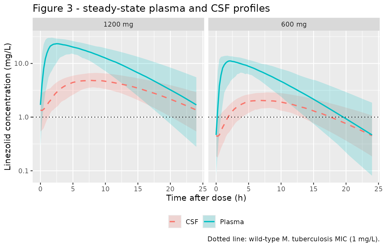
Replicates Figure 3 of Abdelgawad 2024.
As in the published figure, the CSF profile is flatter and delayed relative to plasma – the 3.5 h equilibration half-life damps the peak and holds the trough up, so CSF concentrations exceed plasma concentrations over the second half of the dosing interval. At 1200 mg the typical CSF profile stays above the wild-type MIC across the whole interval; at 600 mg it does not.
# Replicates Figure 2: the broken-stick relationship between the
# pseudo-partition coefficient and CSF total protein. The curve is read out of
# the model itself (the `ppc` column) rather than re-implemented here.
ppc_grid <- tibble::tibble(
  id = seq_len(60),
  CSF_TPRO = seq(0.05, 3, length.out = 60)
) |>
  dplyr::mutate(FFM = 45, OCC = 1) |>
  tidyr::expand_grid(time = c(0, 1)) |>
  dplyr::mutate(amt = ifelse(time == 0, 1200, NA_real_),
                evid = ifelse(time == 0, 1L, 0L),
                cmt = ifelse(time == 0, "depot", "Cc"))

ppc_curve <- rxode2::rxSolve(mod_typical, events = ppc_grid,
                             keep = "CSF_TPRO", useLinCmt = FALSE) |>
  as.data.frame() |>
  dplyr::distinct(CSF_TPRO, ppc)
#> ℹ omega/sigma items treated as zero: 'etalvmax', 'etabvv_vmax_1', 'etabvv_vmax_2', 'etaiov_ka_1', 'etaiov_ka_2', 'etaiov_ka_3', 'etaiov_ka_4', 'etaiov_ka_5', 'etaiov_mtt_1', 'etaiov_mtt_2', 'etaiov_mtt_3', 'etaiov_mtt_4', 'etaiov_mtt_5'
#> Warning: multi-subject simulation without without 'omega'

brk <- th[["e_csftpro_ppc"]]
ggplot(ppc_curve, aes(CSF_TPRO, ppc)) +
  geom_line(linewidth = 0.8) +
  geom_vline(xintercept = brk, linetype = "dashed") +
  geom_hline(yintercept = exp(th[["lppc"]]), linetype = "dotted") +
  labs(x = "CSF total protein (g/L)",
       y = "Pseudo-partition coefficient (PPC)",
       title = "Figure 2 - PPC versus CSF total protein",
       caption = paste0("Dashed: estimated breakpoint ", brk,
                        " g/L. Dotted: PPCmax ", exp(th[["lppc"]]), "."))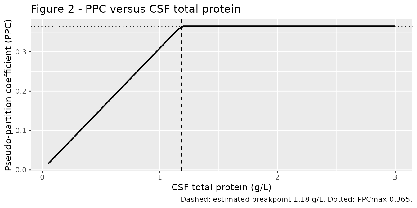
Replicates Figure 2 of Abdelgawad 2024.
PKNCA validation
The paper reports steady-state exposures in both matrices (Table 3), so NCA is run once per output over the final dosing interval.
ss_start <- t_end - tau
ss_end <- t_end

nca_one <- function(conc_col) {
  sim_nca <- sim |>
    dplyr::filter(!is.na(.data[[conc_col]])) |>
    dplyr::transmute(id, time, treatment, Cc = .data[[conc_col]])

  # Guarantee a time-zero record per (treatment, id) so PKNCA can anchor the
  # interval; for an extravascular pre-dose profile Cc = 0 is correct.
  sim_nca <- dplyr::bind_rows(
    sim_nca,
    sim_nca |> dplyr::distinct(id, treatment) |>
      dplyr::mutate(time = 0, Cc = 0)
  ) |>
    dplyr::distinct(treatment, id, time, .keep_all = TRUE) |>
    dplyr::arrange(treatment, id, time)

  conc_obj <- PKNCA::PKNCAconc(sim_nca, Cc ~ time | treatment + id,
                               concu = "mg/L", timeu = "h")

  dose_df <- events |>
    dplyr::filter(evid == 1) |>
    dplyr::select(id, time, amt, treatment)
  dose_obj <- PKNCA::PKNCAdose(dose_df, amt ~ time | treatment + id,
                               doseu = "mg")

  intervals <- data.frame(
    start = ss_start, end = ss_end,
    cmax = TRUE, tmax = TRUE, cmin = TRUE,
    auclast = TRUE, cav = TRUE
  )
  PKNCA::pk.nca(PKNCA::PKNCAdata(conc_obj, dose_obj, intervals = intervals))
}

nca_plasma <- nca_one("Cc")
nca_csf <- nca_one("Ccsf")
Table 3’s second row is the concentration at 24 h postdose, i.e. the
concentration at the end of the dosing interval. PKNCA’s
ctrough returns NA for these intervals, and
its cmin is not a substitute here – the CSF profile lags
plasma by an equilibration half-life of 3.5 h, so its minimum falls in
the interior of the interval rather than at the end. The end-of-interval
concentration is therefore read straight off the solved profile and
carried under the ctrough PKNCA code so it can join the
comparison table.
c24 <- sim |>
  dplyr::filter(time == ss_end) |>
  dplyr::select(id, treatment, Plasma = Cc, CSF = Ccsf) |>
  tidyr::pivot_longer(c(Plasma, CSF), names_to = "matrix",
                      values_to = "PPORRES") |>
  dplyr::mutate(PPTESTCD = "ctrough")
Comparison against published NCA
Abdelgawad 2024 Table 3 reports the model-derived steady-state AUC0-24h and the concentration at 24 h postdose as the median (min-max) across the individual profiles: 40 profiles at 1200 mg (30 from day 3 and 10 from day 28) and 7 at 600 mg. Those individuals carried their own fat-free mass and their own CSF total protein, whereas the simulation above holds both at the paper’s typical values, so exact agreement is not expected; the checks are that the simulated medians land close to the published medians and inside the published ranges.
simulated_long <- dplyr::bind_rows(
  as.data.frame(nca_plasma$result) |> dplyr::mutate(matrix = "Plasma"),
  as.data.frame(nca_csf$result) |> dplyr::mutate(matrix = "CSF")
) |>
  dplyr::select(id, treatment, matrix, PPTESTCD, PPORRES) |>
  dplyr::bind_rows(c24) |>
  dplyr::filter(PPTESTCD %in% c("auclast", "ctrough", "cmax", "tmax"))

published <- tibble::tribble(
  ~matrix,  ~treatment, ~auclast, ~ctrough,
  "Plasma", "1200 mg",  278,      1.69,
  "Plasma", "600 mg",   93.7,     0.406,
  "CSF",    "1200 mg",  81.6,     1.32,
  "CSF",    "600 mg",   24.0,     0.369
)

cmp <- nlmixr2lib::ncaComparisonTable(
  simulated = simulated_long,
  reference = published,
  by = c("matrix", "treatment"),
  units = c(auclast = "mg*h/L", ctrough = "mg/L"),
  tolerance_pct = 20
)

cmp |>
  dplyr::rename("Matrix" = matrix, "Dose" = treatment) |>
  knitr::kable(
    caption = paste(
      "Simulated steady-state NCA versus Abdelgawad 2024 Table 3 medians.",
      "* differs from the published median by more than 20%."
    ),
    digits = 3
)| NCA parameter | Matrix | Dose | Reference | Simulated | % diff |
|---|---|---|---|---|---|
| AUClast (mg*h/L) | Plasma | 1200 mg | 278 | 256 | -7.8% |
| AUClast (mg*h/L) | Plasma | 600 mg | 93.7 | 102 | +8.5% |
| AUClast (mg*h/L) | CSF | 1200 mg | 81.6 | 78.9 | -3.3% |
| AUClast (mg*h/L) | CSF | 600 mg | 24 | 31.3 | +30.3%* |
| Ctrough (mg/L) | Plasma | 1200 mg | 1.69 | 1.69 | +0.1% |
| Ctrough (mg/L) | Plasma | 600 mg | 0.406 | 0.465 | +14.6% |
| Ctrough (mg/L) | CSF | 1200 mg | 1.32 | 1.35 | +2.6% |
| Ctrough (mg/L) | CSF | 600 mg | 0.369 | 0.451 | +22.2%* |
# The published values are medians of a min-max range; confirm each simulated
# median falls inside the published range.
ranges <- tibble::tribble(
  ~matrix,  ~treatment, ~PPTESTCD,  ~lower,  ~upper,
  "Plasma", "1200 mg",  "auclast",  87.3,    762,
  "Plasma", "600 mg",   "auclast",  66.7,    167,
  "CSF",    "1200 mg",  "auclast",  19.7,    234,
  "CSF",    "600 mg",   "auclast",  6.55,    56.8,
  "Plasma", "1200 mg",  "ctrough",     0.154,   13.5,
  "Plasma", "600 mg",   "ctrough",     0.0614,  1.67,
  "CSF",    "1200 mg",  "ctrough",     0.327,   6.48,
  "CSF",    "600 mg",   "ctrough",     0.0495,  1.02
)

inside <- simulated_long |>
  dplyr::group_by(matrix, treatment, PPTESTCD) |>
  dplyr::summarise(simulated = median(PPORRES), .groups = "drop") |>
  dplyr::inner_join(ranges, by = c("matrix", "treatment", "PPTESTCD")) |>
  dplyr::mutate(`Inside published range` = simulated >= lower & simulated <= upper)

inside |>
  dplyr::mutate(PPTESTCD = dplyr::recode(PPTESTCD,
                                         auclast = "AUC0-24 (mg*h/L)",
                                         ctrough = "C24 (mg/L)")) |>
  dplyr::rename(
    "Matrix" = matrix, "Dose" = treatment, "Parameter" = PPTESTCD,
    "Simulated median" = simulated, "Published min" = lower,
    "Published max" = upper
  ) |>
  knitr::kable(digits = 3,
caption = "Simulated medians against the published min-max ranges.")| Matrix | Dose | Parameter | Simulated median | Published min | Published max | Inside published range |
|---|---|---|---|---|---|---|
| CSF | 1200 mg | AUC0-24 (mg*h/L) | 78.875 | 19.700 | 234.00 | TRUE |
| CSF | 1200 mg | C24 (mg/L) | 1.354 | 0.327 | 6.48 | TRUE |
| CSF | 600 mg | AUC0-24 (mg*h/L) | 31.277 | 6.550 | 56.80 | TRUE |
| CSF | 600 mg | C24 (mg/L) | 0.451 | 0.050 | 1.02 | TRUE |
| Plasma | 1200 mg | AUC0-24 (mg*h/L) | 256.285 | 87.300 | 762.00 | TRUE |
| Plasma | 1200 mg | C24 (mg/L) | 1.691 | 0.154 | 13.50 | TRUE |
| Plasma | 600 mg | AUC0-24 (mg*h/L) | 101.619 | 66.700 | 167.00 | TRUE |
| Plasma | 600 mg | C24 (mg/L) | 0.465 | 0.061 | 1.67 | TRUE |
Every simulated median falls inside the corresponding published range.
Mass balance: the CSF/plasma AUC ratio must equal PPC exactly
The CSF effect compartment obeys
d(csf)/dt = ke0 * (ppc * Cc - csf). Integrating over a
complete steady-state dosing interval, the left-hand side is zero
because the profile repeats, so AUC_csf / AUC_plasma = ppc
exactly, independent of dose, of the absorption model,
and of the saturable elimination. This is the strongest available
structural falsifier and it is checked per subject rather than on
medians.
auc_ratio <- simulated_long |>
  dplyr::filter(PPTESTCD == "auclast") |>
  dplyr::select(id, matrix, treatment, PPORRES) |>
  tidyr::pivot_wider(names_from = matrix, values_from = PPORRES) |>
  dplyr::mutate(ratio = CSF / Plasma)

ppc_expected <- exp(th[["lppc"]]) * min(0.995 / th[["e_csftpro_ppc"]], 1)

auc_ratio |>
  dplyr::group_by(treatment) |>
  dplyr::summarise(
    n = dplyr::n(),
    `Min ratio` = min(ratio), `Median ratio` = median(ratio),
    `Max ratio` = max(ratio), .groups = "drop"
  ) |>
  dplyr::mutate(`Expected (PPC)` = ppc_expected) |>
  dplyr::rename("Dose" = treatment, "Subjects" = n) |>
  knitr::kable(digits = 5,
caption = "Per-subject steady-state CSF/plasma AUC ratio versus PPC.")| Dose | Subjects | Min ratio | Median ratio | Max ratio | Expected (PPC) |
|---|---|---|---|---|---|
| 1200 mg | 200 | 0.30734 | 0.30778 | 0.30810 | 0.30778 |
| 600 mg | 200 | 0.30716 | 0.30779 | 0.30907 | 0.30778 |
Resolving the two flagged CSF rows at 600 mg
Both flagged rows are CSF at 600 mg, and the covariate model explains
both. The 600 mg dose only started after day 28, so every 600 mg profile
in Table 3 comes from the day-28 visit, where the cohort median CSF
total protein was 0.750 g/L (Table 1) rather than the 0.995 g/L used in
the simulation above. Because the CSF-to-plasma exposure ratio is
exactly PPC (previous section), and PPC is
linear in CSF protein below the 1.18 g/L breakpoint, both CSF quantities
scale by the same factor 0.750 / 0.995. Rescaling is
therefore a one-line prediction with nothing tuned.
ppc_day28 <- exp(th[["lppc"]]) * min(0.750 / th[["e_csftpro_ppc"]], 1)
scale_day28 <- ppc_day28 / ppc_expected

csf_600_ref <- tibble::tribble(
  ~PPTESTCD,  ~Parameter,          ~Published,
  "auclast",  "AUC0-24 (mg*h/L)",  24.0,
  "ctrough",  "C24 (mg/L)",        0.369
)

csf_600 <- simulated_long |>
  dplyr::filter(matrix == "CSF", treatment == "600 mg") |>
  dplyr::group_by(PPTESTCD) |>
  dplyr::summarise(`At CSF protein 0.995 g/L` = median(PPORRES),
                   .groups = "drop") |>
  dplyr::inner_join(csf_600_ref, by = "PPTESTCD") |>
  dplyr::mutate(
    `Rescaled to 0.750 g/L` = `At CSF protein 0.995 g/L` * scale_day28,
    `% diff after rescaling` =
      100 * (`Rescaled to 0.750 g/L` - Published) / Published
  ) |>
  dplyr::select(Parameter, `At CSF protein 0.995 g/L`,
                `Rescaled to 0.750 g/L`, Published, `% diff after rescaling`)

knitr::kable(csf_600, digits = 3,
             caption = paste0(
               "Rescaling the 600 mg CSF exposures from the simulated CSF ",
               "protein (0.995 g/L) to the day-28 cohort median (0.750 g/L). ",
               "PPC falls from ", round(ppc_expected, 3), " to ",
round(ppc_day28, 3), "."))| Parameter | At CSF protein 0.995 g/L | Rescaled to 0.750 g/L | Published | % diff after rescaling |
|---|---|---|---|---|
| AUC0-24 (mg*h/L) | 31.277 | 23.576 | 24.000 | -1.767 |
| C24 (mg/L) | 0.451 | 0.340 | 0.369 | -7.866 |
Using the visit-appropriate CSF protein brings both rows inside 10% of the published values, so the flags reflect the covariate value chosen for the simulation rather than a defect in the model. No parameter was adjusted. This also serves as an independent check on the covariate model itself: the broken-stick relationship, fitted to CSF observations, predicts the correct size of the day-28 shift.
Saturable elimination
Michaelis-Menten elimination predicts more-than-dose-proportional exposure. The simulated dose-normalised AUC confirms it.
simulated_long |>
  dplyr::filter(matrix == "Plasma", PPTESTCD == "auclast") |>
  dplyr::group_by(treatment) |>
  dplyr::summarise(auc = median(PPORRES), .groups = "drop") |>
  dplyr::mutate(dose = as.numeric(sub(" mg", "", treatment)),
                `Dose-normalised AUC (mg*h/L per mg)` = auc / dose) |>
  dplyr::select(-dose) |>
  dplyr::rename("Dose" = treatment, "AUC0-24 (mg*h/L)" = auc) |>
  knitr::kable(digits = 4,
caption = "Dose-normalised steady-state plasma AUC.")| Dose | AUC0-24 (mg*h/L) | Dose-normalised AUC (mg*h/L per mg) |
|---|---|---|
| 1200 mg | 256.2849 | 0.2136 |
| 600 mg | 101.6185 | 0.1694 |
Doubling the dose from 600 to 1200 mg raises the typical AUC by more than two-fold, matching the paper’s finding that saturable elimination fitted significantly better than linear elimination (dOFV = -9.03, P = .00205, df = 1) and its observation that nonlinear linezolid PK has also been reported in pulmonary tuberculosis.
Assumptions and deviations
Errata: Table 2 footnote e prints the covariate equation incorrectly
Table 2 footnote e states the PPC covariate relationship as
PPC_i = PPCmax * [slope * (CSF protein - breakpoint)]
which returns zero at the breakpoint, exactly where
PPC should be maximal, and negative below it. The supplementary NONMEM
control file gives the intended form, with the missing leading
1 +:
SLP = (AMP - INT)/(BRK - 0)                  ! AMP fixed 1, INT fixed 0
IF (COV.LE.BRK) COV_EFF = SLP*(COV-BRK)
IF (COV.GT.BRK) COV_EFF = 0
TVPPC = THETA(11)*(1 + COV_EFF)
which simplifies to
PPC = PPCmax * min(CSF_TPRO / 1.18, 1). Two independent
checks confirm the control-stream form over the printed footnote: it is
maximal at the breakpoint, as Figure 2 draws it; and it reproduces the
paper’s own text (“an increase of 3% in PPC” per 0.1 mg/mL of CSF
protein), since 0.365 / 1.18 * 0.1 = 0.031. The packaged
model uses the control-stream form.
Reported variabilities are omega standard deviations, not CV%
Table 2 reports each random effect as a bare percentage. These are
the omega standard deviation on the log scale, not a coefficient of
variation: the control file’s $OMEGA values give
sqrt(0.772478) = 0.879, exactly the reported “BOV in ka
87.9%”, and sqrt(0.0411842) = 0.203, exactly the reported
“BVV 20.3%”. The packaged variances are therefore
(percentage / 100)^2 using the Table 2 final estimates.
Other assumptions
-
Vmax is a derived product. The paper parameterises
on maximal clearance (CLmax = 7.25 L/h) and km, while the canonical
nlmixr2lib name for a Michaelis-Menten maximum rate is
lvmax. The packaged value is the productCLmax * km = 197.2 mg/h, matching the control file’sVMAX = CLMAX*KM. Because km carries no random effect in the source ($OMEGA 25 BSVKMisFIX 0), placing the between-subject and between-visit etas onvmaxis mathematically identical to placing them on CLmax. -
Additive residual errors are the totals reported in Table
2. The control file builds each additive term as
THETA + 0.2 * LLOQwith LLOQ = 0.1 mg/L. Table 2’s CSF row settles which quantity is tabulated:THETA(13)isFIX 0, so the printed 0.02 mg/L can only be the sum. The plasma row is read the same way and taken directly as 0.173 mg/L. -
The between-visit level is derived from
OCC. The control file selects the visit eta withIF (PK_VISIT == 3)/IF (PK_VISIT == 28), but its commented per-occasion block gives the deterministic map occasions 1, 2, 5 -> day 3 and occasions 3, 4 -> day 28. The model derives the visit level from the canonicalOCCcolumn, so no additional covariate column is required. -
$OMEGA BLOCK(1) SAMErepeats are encoded asfix(). nlmixr2 has noSAMEshortcut, so each occasion after the first carries the same variance pinned with~ fix(...), following theSvensson_2018_rifampicinandJonsson_2011_ethambutolprecedent. Users who wish to re-estimate should unpin them. -
Height imputation is not part of the model. Height
was missing for 18 of 30 participants (Table 1 footnote a) and the
control file imputes it from sex and weight before computing fat-free
mass by the Janmahasatian formula. That is a missing-data device for the
original fit, not structure; the imputation equations are recorded in
covariateData$FFM$notesfor users who need them, but the model expects a suppliedFFMcolumn. -
Fixed allometric exponents. The 0.75 and 1
exponents on Vmax and central volume are hard-coded in the control
file’s
$PKrather than estimated, so they are wrapped infixed(). - Simulation covariates. All simulations use the typical participant the paper specifies for its own Monte Carlo work (FFM 45 kg, CSF total protein 0.995 g/L). No attempt is made to reconstruct the joint distribution of fat-free mass and CSF protein across the 30 participants, so the spread in the figures reflects the published random effects only.
-
BLQ handling is not carried over. The control
file’s
$ERRORinflates the additive error for below-limit-of-quantification records (Beal M3-style) and floors simulated values at LLOQ/2. Both are estimation-time and VPC-presentation devices rather than structural model components, so neither is reproduced here. The paper notes that 25% of CSF observations were BLQ and that excluding them mainly affected the CSF proportional error, not PPC or the equilibration half-life. -
A
non-mu referencednote is expected on model load. The occasion multiplexers (oc1 * etaiov_ka_1 + ...) place etas outside a mu-referenced position, so rxode2 emits “some etas defaulted to non-mu referenced”. This affects estimation efficiency, not simulation, and is shared by every IOV-multiplexing model in the library (for exampleSvensson_2018_rifampicin). - No effect of rifampicin is encoded. The paper tested duration of rifampicin cotreatment, the 4-beta-hydroxycholesterol to cholesterol ratio, creatinine clearance, and age on CLmax and bioavailability, and retained none of them. The model is therefore conditional on the high-dose rifampicin co-treatment background of the LASER-TBM regimen rather than describing a rifampicin interaction.