Model and source
- Citation: Senek M, Nyholm D, Nielsen EI. Population pharmacokinetics of levodopa gel infusion in Parkinson’s disease: effects of entacapone infusion and genetic polymorphism. Sci Rep. 2020;10:18057. doi:10.1038/s41598-020-75052-2
- Description: One-compartment population PK model for levodopa given as an intrajejunal gel infusion (levodopa-carbidopa intestinal gel, LCIG, or levodopa-entacapone-carbidopa intestinal gel, LECIG) in advanced Parkinson’s disease, with fixed fast first-order absorption from the jejunum, a one-transit-compartment absorption branch for night-time oral levodopa-carbidopa tablets, allometric body-weight scaling of CL/F and V/F, and a fractional shift in CL/F (with its own IIV) during simultaneous entacapone infusion (Senek 2020)
- Article: https://doi.org/10.1038/s41598-020-75052-2 (open access)
Levodopa-carbidopa intestinal gel (LCIG) and levodopa-entacapone-carbidopa intestinal gel (LECIG) are infused directly into the jejunum through a gastrojejunostomy tube as a morning bolus followed by a continuous maintenance infusion. Senek 2020 fitted a population PK model to a two-day LCIG/LECIG crossover to find the LECIG dose that matches LCIG exposure. Adding entacapone lowered levodopa CL/F by 36.5%, and the authors concluded that the continuous maintenance dose should be reduced by about 35% when switching to LECIG.
Population
Eleven patients with advanced Parkinson’s disease on established LCIG therapy (7 male, 4 female) were studied in a randomised, open-label, two-day crossover (Senek 2020 Table 1): age 63-76 years (median 70), body weight 51-99 kg (median 73, mean 74, SD 15), PD duration 8-23 years, LCIG duration 0.2-7.6 years. LCIG morning doses were 41-217 mg (mean 131) and continuous maintenance doses 363-1367 mg (mean 969) of levodopa over a 14-hour infusion day. On the LECIG day the morning dose was 80% (n = 5) or 90% (n = 6) of the LCIG morning dose and the maintenance and extra-bolus doses were 80% of LCIG. At 14 h the tube was flushed, delivering about 3 mL of gel (60 mg levodopa). Oral levodopa-carbidopa tablets were allowed at night until 3 h before the infusion.
The same information is available programmatically via
readModelDb("Senek_2020_levodopa")()$population.
Source trace
Every ini() value carries an in-file comment in
inst/modeldb/specificDrugs/Senek_2020_levodopa.R; the table
collects them.
| Equation / parameter | Value | Source location |
|---|---|---|
| One-compartment disposition, first-order absorption | – | Results, first paragraph |
lka (ka) |
fixed(log(50)) 1/h |
Table 2; Results (“fixed to 50 h-1”) |
lcl (CL/F, LCIG, 70 kg) |
log(27.9) L/h |
Table 2 |
lvc (V/F, 70 kg) |
log(74.5) L |
Table 2 (abstract prints 74.4) |
lfdepot (Frel gel) |
fixed(log(1)) |
Table 2 |
Oral tablet branch: depot -> one transit -> central, common
rate ktr
|
– | Methods, “Model development” (taken from Othman 2014) |
lktr |
fixed(log(2.4)) 1/h |
Table 2 |
lfdepot_oral (Frel oral) |
fixed(log(1.03)) |
Table 2 |
e_wt_cl, e_wt_vc
|
fixed(0.75), fixed(1)
|
Methods, “Model development” |
CL/F shift equation
CL = TVCL * exp(eta_CL) * (WT/70)^0.75 * (1 + shift * exp(eta_shift))
|
– | Table 2 footnote a |
e_conmed_entacapone_cl (shift) |
-0.365 | Table 2 |
etalcl |
0.07497 (27.9% CV) | Table 2 |
etae_conmed_entacapone_cl |
0.01291 (11.4% CV) | Table 2 |
etalvc |
0.1118 (34.4% CV) | Table 2 |
propSd |
0.110 | Table 2 |
addSd |
0.316 ug/mL | Table 2 |
Typical-value checks
The model is linear, so at steady state a constant jejunal infusion
at rate R gives Css = R / CL for any
absorption rate. The LECIG clearance for a 70 kg patient is
27.9 * (1 - 0.365), which the Discussion prints as 17.7
L/h/70 kg. Both follow from a deterministic solve with the random
effects zeroed.
mod <- readModelDb("Senek_2020_levodopa")
mod_typ <- rxode2::zeroRe(mod)
#> ℹ parameter labels from comments will be replaced by 'label()'

rate <- 70 # mg/h, a typical LCIG maintenance rate
ev_ss <- rxode2::et(amt = rate * 100, rate = rate, cmt = "depot") |>
  rxode2::et(seq(0, 100, by = 1), cmt = "central")

css <- function(entacapone, wt = 70) {
  s <- rxode2::rxSolve(mod_typ, ev_ss,
    params = data.frame(WT = wt, CONMED_ENTACAPONE = entacapone)
  )
  s$Cc[s$time == 99]
}
css_lcig <- css(0)
#> ℹ omega/sigma items treated as zero: 'etalcl', 'etae_conmed_entacapone_cl', 'etalvc'
css_lecig <- css(1)
#> ℹ omega/sigma items treated as zero: 'etalcl', 'etae_conmed_entacapone_cl', 'etalvc'
cl_lecig <- rate / css_lecig

data.frame(
  quantity = c("Css LCIG (ug/mL)", "Css LECIG (ug/mL)", "CL/F LECIG, 70 kg (L/h)"),
  simulated = signif(c(css_lcig, css_lecig, cl_lecig), 4),
  expected = signif(c(rate / 27.9, rate / (27.9 * (1 - 0.365)), 17.7), 4)
) |> knitr::kable()| quantity | simulated | expected |
|---|---|---|
| Css LCIG (ug/mL) | 2.509 | 2.509 |
| Css LECIG (ug/mL) | 3.951 | 3.951 |
| CL/F LECIG, 70 kg (L/h) | 17.720 | 17.700 |
stopifnot(
  abs(css_lcig / (rate / 27.9) - 1) < 1e-3,
  abs(cl_lecig - 17.7) < 0.05,
  # allometric exponent 0.75 on CL: a 35 kg patient has (0.5)^0.75 of the CL
  abs(css(0, wt = 35) / css_lcig - 0.5^-0.75) < 1e-3
)
#> ℹ omega/sigma items treated as zero: 'etalcl', 'etae_conmed_entacapone_cl', 'etalvc'
The paper’s dose recommendation follows directly: a 35% lower
maintenance rate on LECIG gives a steady state
0.65 / 0.635 = 1.024 times the LCIG level.
ratio_35 <- 0.65 * css_lecig / css_lcig
ratio_35
#> [1] 1.023622
stopifnot(abs(ratio_35 - 0.65 / 0.635) < 1e-3)
The oral-tablet branch (depot, one transit compartment, 2.4 1/h,
relative bioavailability 1.03) is checked by mass balance: a single 100
mg tablet dose must give AUC(0-inf) = 1.03 * 100 / CL.
ev_oral <- rxode2::et(amt = 100, cmt = "depot_oral") |>
  rxode2::et(c(seq(0, 2, by = 0.05), seq(2.25, 48, by = 0.25)), cmt = "central")
s_oral <- as.data.frame(rxode2::rxSolve(mod_typ, ev_oral,
  params = data.frame(WT = 70, CONMED_ENTACAPONE = 0)
))
#> ℹ omega/sigma items treated as zero: 'etalcl', 'etae_conmed_entacapone_cl', 'etalvc'
auc_oral <- sum(diff(s_oral$time) *
  (head(s_oral$Cc, -1) + tail(s_oral$Cc, -1)) / 2)
c(simulated = auc_oral, expected = 1.03 * 100 / 27.9)
#> simulated  expected
#>  3.692671  3.691756
stopifnot(abs(auc_oral / (1.03 * 100 / 27.9) - 1) < 0.01)
Virtual cohort
Figure 2 of Senek 2020 simulates the study population’s own doses. The individual doses are not published, so the cohort below draws body weight from the Table 1 mean and SD (redrawn until inside the observed 51-99 kg range) and uses the Table 1 LCIG means for every subject: a 131 mg morning bolus at the maximum pump rate (40 mL/h of a 20 mg/mL gel, 800 mg/h), a 969 mg continuous maintenance dose over the rest of the 14-hour day, and a 60 mg flush at 14 h. Extra doses and night-time tablets are omitted.
set.seed(2020)
rxode2::rxSetSeed(2020)
n_sub <- 200

draw_wt <- function(n) {
  wt <- numeric(0)
  while (length(wt) < n) {
    x <- rnorm(n, 74, 15)
    wt <- c(wt, x[x >= 51 & x <= 99])
  }
  wt[seq_len(n)]
}
wt <- draw_wt(n_sub)

scenarios <- tibble::tribble(
  ~scenario, ~entacapone, ~morning_frac, ~maint_frac,
  "LCIG (reference)", 0, 1.00, 1.00,
  "LECIG, 0% lower morning, 35% lower maintenance", 1, 1.00, 0.65,
  "LECIG, 0% lower morning and maintenance", 1, 1.00, 1.00,
  "LECIG, 20% lower morning and maintenance", 1, 0.80, 0.80
)

make_events <- function(i, sc) {
  morning <- 131 * sc$morning_frac
  t_morning <- morning / 800
  maint <- 969 * sc$maint_frac
  obs <- sort(unique(c(seq(0, 17, by = 0.25), 14)))
  id <- (i - 1) * n_sub + seq_len(n_sub)
  dose <- tidyr::expand_grid(id = id, row = 1:3) |>
    mutate(
      time = c(0, t_morning, 14)[row],
      amt = c(morning, maint, 60)[row],
      rate = c(800, maint / (14 - t_morning), 0)[row],
      evid = 1, cmt = "depot"
    ) |>
    select(-row)
  obs_rows <- tidyr::expand_grid(id = id, time = obs) |>
    mutate(amt = 0, rate = 0, evid = 0, cmt = "central")
  bind_rows(dose, obs_rows) |>
    mutate(
      WT = wt[(id - 1) %% n_sub + 1],
      CONMED_ENTACAPONE = sc$entacapone,
      scenario = sc$scenario
    ) |>
    arrange(id, time, desc(evid))
}

events <- bind_rows(lapply(seq_len(nrow(scenarios)), function(i) {
  make_events(i, scenarios[i, ])
}))
Simulation and Figure 2
sim <- rxode2::rxSolve(mod, events,
  keep = c("scenario", "WT", "CONMED_ENTACAPONE"),
  returnType = "data.frame"
)
#> ℹ parameter labels from comments will be replaced by 'label()'
sim_sum <- sim |>
  group_by(scenario, time) |>
  summarise(
    p10 = quantile(Cc, 0.1), p50 = median(Cc), p90 = quantile(Cc, 0.9),
    .groups = "drop"
  ) |>
  mutate(scenario = factor(scenario, levels = scenarios$scenario))

ggplot(sim_sum, aes(time)) +
  geom_line(aes(y = p50)) +
  geom_line(aes(y = p10), linetype = "dashed") +
  geom_line(aes(y = p90), linetype = "dashed") +
  facet_wrap(~scenario) +
  labs(x = "Time after infusion start (h)", y = "Levodopa (ug/mL)")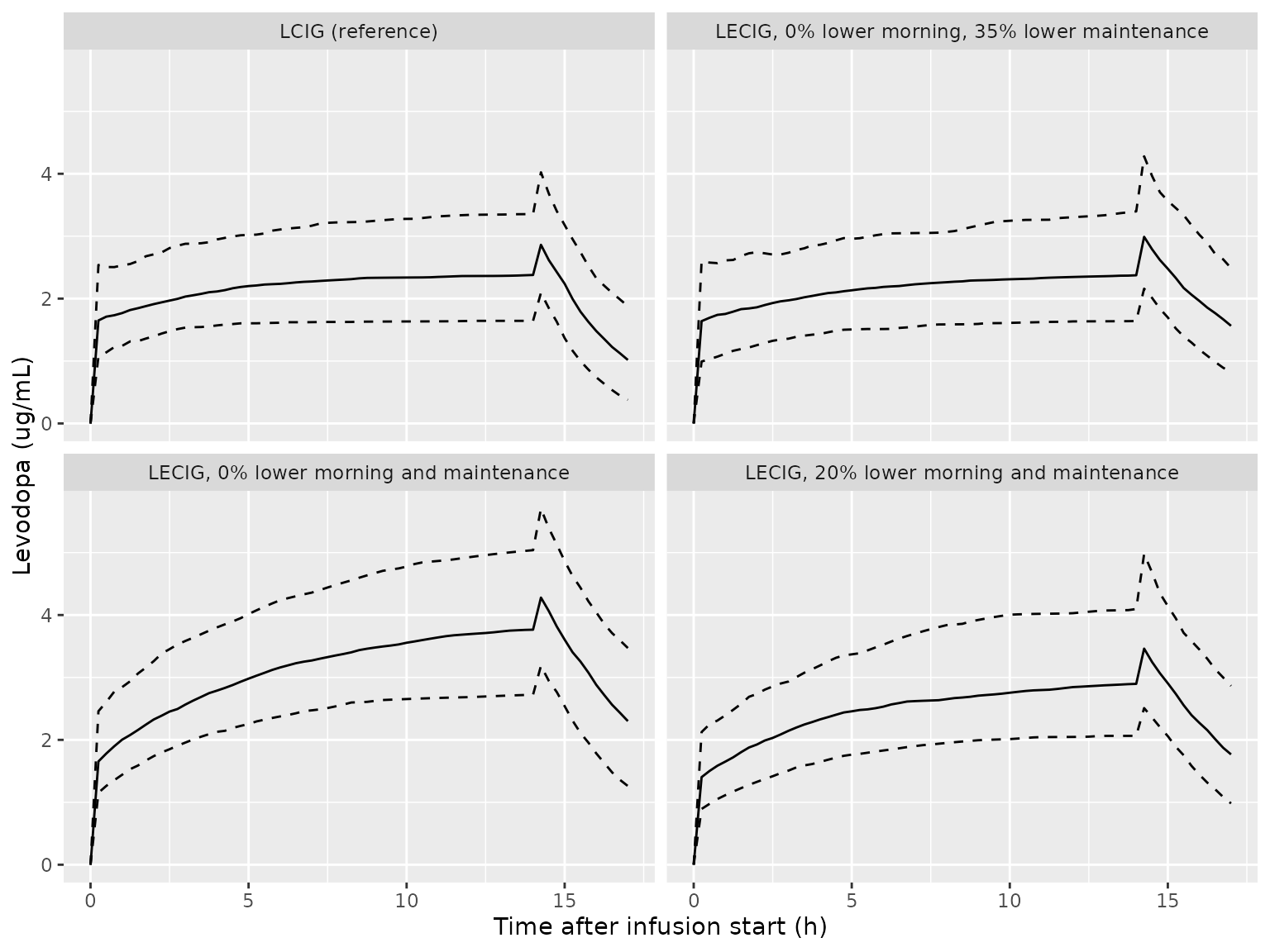
Replicates Figure 2 of Senek 2020: median (solid) and 10th/90th percentiles (dashed) of simulated levodopa plasma concentration for LCIG and three LECIG dose scenarios.
Figure 2 of the paper shows the LECIG concentrations rising through the infusion day at unchanged or 20%-reduced doses and matching LCIG once the maintenance dose is cut by 35%. The simulated median concentration at the end of the infusion day (14 h, just before the flush) reproduces this ordering.
end_day <- sim |>
  filter(time == 14) |>
  group_by(scenario) |>
  summarise(median_Cc = median(Cc), .groups = "drop")
ref <- end_day$median_Cc[end_day$scenario == "LCIG (reference)"]
end_day <- end_day |>
  mutate(ratio_to_LCIG = median_Cc / ref)
end_day |>
  dplyr::rename(
    "Scenario" = scenario,
    "Median Cc at 14 h (ug/mL)" = median_Cc,
    "Ratio to LCIG" = ratio_to_LCIG
  ) |>
knitr::kable(digits = 3)| Scenario | Median Cc at 14 h (ug/mL) | Ratio to LCIG |
|---|---|---|
| LCIG (reference) | 2.379 | 1.000 |
| LECIG, 0% lower morning and maintenance | 3.765 | 1.583 |
| LECIG, 0% lower morning, 35% lower maintenance | 2.374 | 0.998 |
| LECIG, 20% lower morning and maintenance | 2.897 | 1.218 |
r <- setNames(end_day$ratio_to_LCIG, end_day$scenario)
stopifnot(
  # 35% lower maintenance matches LCIG (typical-value ratio 1.024)
  abs(r[["LECIG, 0% lower morning, 35% lower maintenance"]] - 1) < 0.15,
  # unchanged dose: about 1 / 0.635 = 1.57 times LCIG
  abs(r[["LECIG, 0% lower morning and maintenance"]] - 1 / 0.635) < 0.15,
  # the study's 20% reduction: about 0.8 / 0.635 = 1.26 times LCIG
  abs(r[["LECIG, 20% lower morning and maintenance"]] - 0.8 / 0.635) < 0.15
)
PKNCA validation
NCA over the 14-hour infusion day, grouped by scenario. The paper
reports no NCA table, so the check is the AUC(0-14) ratio of each LECIG
scenario to LCIG. Over a finite window this ratio is smaller than the
clearance ratio 1 / 0.635, because the slower LECIG
clearance leaves more levodopa in the body at 14 h. The expected ratio
therefore comes from a typical-value (70 kg, no random effects) solve of
the same regimens, and the cohort median must agree with it.
conc <- sim |>
  filter(!is.na(Cc), time <= 14) |>
  select(id, time, Cc, scenario)
dose_nca <- events |>
  filter(evid == 1, time == 0) |>
  select(id, time, amt, scenario)

o_conc <- PKNCA::PKNCAconc(conc, Cc ~ time | scenario + id,
  concu = "ug/mL", timeu = "h"
)
o_dose <- PKNCA::PKNCAdose(dose_nca, amt ~ time | scenario + id, doseu = "mg")
intervals <- data.frame(start = 0, end = 14, auclast = TRUE, cmax = TRUE)
nca <- PKNCA::pk.nca(PKNCA::PKNCAdata(o_conc, o_dose, intervals = intervals))

nca_tab <- as.data.frame(nca$result) |>
  group_by(scenario, PPTESTCD) |>
  summarise(median = median(PPORRES), .groups = "drop") |>
  tidyr::pivot_wider(names_from = PPTESTCD, values_from = median)
nca_tab |>
  dplyr::rename("Scenario" = scenario, "AUC0-14 (h*ug/mL)" = auclast, "Cmax (ug/mL)" = cmax) |>
knitr::kable(digits = 2)| Scenario | AUC0-14 (h*ug/mL) | Cmax (ug/mL) |
|---|---|---|
| LCIG (reference) | 30.54 | 2.44 |
| LECIG, 0% lower morning and maintenance | 43.20 | 3.78 |
| LECIG, 0% lower morning, 35% lower maintenance | 29.94 | 2.47 |
| LECIG, 20% lower morning and maintenance | 34.66 | 2.90 |
typ_events <- events |>
  filter(id %in% ((seq_len(nrow(scenarios)) - 1) * n_sub + 1)) |>
  mutate(WT = 70)
typ <- rxode2::rxSolve(mod_typ, typ_events,
  keep = "scenario", returnType = "data.frame"
) |>
  filter(time <= 14) |>
  group_by(scenario) |>
  summarise(
    auc_typ = sum(diff(time) * (head(Cc, -1) + tail(Cc, -1)) / 2),
    .groups = "drop"
  )
#> ℹ omega/sigma items treated as zero: 'etalcl', 'etae_conmed_entacapone_cl', 'etalvc'
#> Warning: multi-subject simulation without without 'omega'

auc_cmp <- nca_tab |>
  select(scenario, auclast) |>
  left_join(typ, by = "scenario") |>
  mutate(
    ratio_sim = auclast / auclast[scenario == "LCIG (reference)"],
    ratio_typ = auc_typ / auc_typ[scenario == "LCIG (reference)"]
  )
auc_cmp |>
  dplyr::rename(
    "Scenario" = scenario,
    "Median AUC0-14, cohort" = auclast,
    "AUC0-14, typical 70 kg" = auc_typ,
    "Ratio to LCIG, cohort" = ratio_sim,
    "Ratio to LCIG, typical" = ratio_typ
  ) |>
knitr::kable(digits = 3)| Scenario | Median AUC0-14, cohort | AUC0-14, typical 70 kg | Ratio to LCIG, cohort | Ratio to LCIG, typical |
|---|---|---|---|---|
| LCIG (reference) | 30.536 | 32.644 | 1.000 | 1.000 |
| LECIG, 0% lower morning and maintenance | 43.200 | 45.697 | 1.415 | 1.400 |
| LECIG, 0% lower morning, 35% lower maintenance | 29.937 | 32.181 | 0.980 | 0.986 |
| LECIG, 20% lower morning and maintenance | 34.657 | 36.563 | 1.135 | 1.120 |
Assumptions and deviations
-
IIV scale. Table 2 reports IIV as CV%; the
variances use the log-normal conversion
omega^2 = log(CV^2 + 1). At 11-34% CV this differs fromCV^2by under 3%. - Shift IIV. Table 2 footnote a places the random effect exponentially on the shift term, so each patient’s shift stays negative; this is encoded as printed.
- Volume. Table 2 (74.5 L/70 kg) is used; the abstract prints 74.4.
-
Entacapone indicator. The shift applies to the
whole LECIG day; the paper does not separate the COMT-inhibition effect
from any gel-formulation effect, so
CONMED_ENTACAPONE = 1stands for “LECIG infusion”. - Figure 2 doses. Individual doses are unpublished; every virtual patient receives the Table 1 mean LCIG doses (131 mg morning, 969 mg maintenance) and a 60 mg flush, without extra boluses or night-time tablets. The paper simulated 1000 replicates of the 11 study patients; this vignette uses 200 subjects per scenario with body weight drawn from Table 1.
- Genotypes. COMT rs4680 and DDC rs921451 / rs3837091 were explored only graphically on empirical Bayes estimates (Figure 3) and are not model covariates.
- Protein intake was tested on absorption and bioavailability but not retained.