Buprenorphine (Kovar 2020)
Source:vignettes/articles/Kovar_2020_buprenorphine.Rmd
Kovar_2020_buprenorphine.RmdModel and source
- Citation: Kovar L, Schrapel C, Selzer D, Kohl Y, Bals R, Schwab M, Lehr T. Physiologically-Based Pharmacokinetic (PBPK) Modeling of Buprenorphine in Adults, Children and Preterm Neonates. Pharmaceutics. 2020;12(6):578. doi:10.3390/pharmaceutics12060578
- Description: Three-compartment intravenous PK model for buprenorphine in adults (typical values fitted in NONMEM to digitised mean literature profiles), scaled to children and preterm neonates by fixed-exponent allometry on body weight (Tod et al. 2008 approach). This is the classical allometric comparator of the Kovar 2020 paper; the paper’s PK-Sim whole-body PBPK model is not included.
- Article: https://doi.org/10.3390/pharmaceutics12060578
- Supplement: https://www.mdpi.com/1999-4923/12/6/578/s1
Kovar et al. built a whole-body parent-metabolite PBPK model of intravenous buprenorphine and norbuprenorphine in PK-Sim, scaled it to children and preterm neonates, and used it for drug-drug interaction simulations. To benchmark the paediatric PBPK predictions they also fitted a classical three-compartment model to the same adult training data in NONMEM and scaled it to the paediatric patients by fixed-exponent allometry (the Tod et al. 2008 approach; Supplementary Materials Section 3, Equations S9-S15, Table S4).
This package entry is that three-compartment allometric model. The PK-Sim PBPK model is not included: its organ volumes, blood flows, tissue partition coefficients (calculated by the Schmitt method inside the software) and enzyme expression profiles are outputs of the PK-Sim database and are not printed in the paper or supplement, so the model cannot be rebuilt from the publication.
Population
The adult parameters were estimated on the internal (training)
dataset of the PBPK analysis (main-text Table 1, studies marked
i): digitised mean intravenous profiles from Bullingham
1982 arm 2 (0.3 mg over 1 min, n = 5, mean age 64.2 years, 66.4 kg),
Everhart 1999 (1 mg over 60 min, n = 6), Huestis 2013 arms 1 and 5 (2
and 16 mg over 1 min, n = 5, 32-39 years, 62.1-82.6 kg) and Kuhlman 1996
(1.2 mg over 1 min, n = 5 men, 27-40 years, 62.6-72.7 kg). Arterial and
venous samples were pooled. The reference adult weight is 71 kg.
The model was then scaled to two external paediatric studies: Olkkola 1989 (10 children aged 4.6-7.5 years, median 21.4 kg, 3 ug/kg over 2 min) and Barrett 1993 (12 ventilated preterm neonates of 27-34 weeks postmenstrual age and 0.9-2.4 kg, 3 ug/kg loading over 30 min followed by 0.72-2.16 ug/kg/h for 11-118 h; Supplementary Table S2).
The same information is available programmatically via
readModelDb("Kovar_2020_buprenorphine")()$population.
Source trace
| Equation / parameter | Value | Source location |
|---|---|---|
lcl |
log(982.0 / 1000) L/min | Supplementary Table S4, ‘Adults (internal dataset)’, CL 982.0 mL/min |
lvc |
log(29.6) L | Table S4, Vc 29.6 L |
lq |
log(2980.0 / 1000) L/min | Table S4, Q2 2980.0 mL/min |
lvp |
log(105.0) L | Table S4, V2 105.0 L |
lq2 |
log(554.0 / 1000) L/min | Table S4, Q3 554.0 mL/min |
lvp2 |
log(676.0) L | Table S4, V3 676.0 L |
e_wt_cl |
0.75 (fixed) | Equation S9; 1.2 for the age-dependent variant in preterm neonates, Equation S15 |
e_wt_q_q2 |
0.75 (fixed) | Equations S10-S11 |
e_wt_vc_vp_vp2 |
1 (fixed) | Equations S12-S14 |
| Reference weight | 71 kg | Supplementary Section 3 (‘adult (71 kg)’) |
| Three-compartment structure, IV input into central | – | Supplementary Section 3 (‘classical three compartment model’) |
Reproducing Table S4
Table S4 lists the allometrically scaled parameters for each paediatric patient. The model’s own scaling equations, evaluated at the body weights of Supplementary Table S2 and main-text Table 1, reproduce it. The body weights are printed to 0.1 kg, which alone moves CL by up to 4 % (exponent 0.75) or 7 % (exponent 1.2) at 0.9 kg, and several volumes are printed to 0.1 L, so the comparison allows for both roundings.
ped <- tibble::tribble(
  ~study, ~WT, ~CL_a, ~CL_b, ~Q2, ~Q3, ~Vc, ~V2, ~V3,
  "Barrett 1993 (1)", 1.5, 54.5, 9.6, 165, 31, 0.6, 2.2, 14.3,
  "Barrett 1993 (2)", 0.9, 37.8, 5.3, 115, 21, 0.4, 1.4, 8.8,
  "Barrett 1993 (3)", 1.3, 50.1, 8.4, 152, 28, 0.6, 2.0, 12.8,
  "Barrett 1993 (4)", 1.8, 61.4, 12.0, 186, 35, 0.7, 2.6, 16.8,
  "Barrett 1993 (5)", 1.5, 54.5, 9.6, 165, 31, 0.6, 2.2, 14.3,
  "Barrett 1993 (6)", 1.2, 44.9, 7.1, 136, 25, 0.5, 1.7, 11.1,
  "Barrett 1993 (7)", 1.1, 44.4, 6.9, 135, 25, 0.5, 1.7, 10.9,
  "Barrett 1993 (8)", 1.8, 61.4, 11.6, 186, 35, 0.7, 2.6, 16.8,
  "Barrett 1993 (9)", 1.6, 56.9, 10.3, 173, 32, 0.7, 2.4, 15.2,
  "Barrett 1993 (10)", 2.4, 77.5, 16.9, 235, 44, 1.0, 3.6, 22.9,
  "Barrett 1993 (11)", 1.6, 56.7, 10.2, 172, 32, 0.7, 2.3, 15.1,
  "Barrett 1993 (12)", 1.0, 41.4, 6.2, 126, 23, 0.4, 1.5, 9.9,
  "Olkkola 1989", 21.4, 400, 400, 1214, 226, 8.9, 32.0, 204
)

mod <- readModelDb("Kovar_2020_buprenorphine")()
p <- as.list(mod$theta)
scale_par <- function(wt, e) (wt / 71)^e
calc <- ped |>
  mutate(
    CL_a_model = 1000 * exp(p$lcl) * scale_par(WT, p$e_wt_cl),
    # Equation S15 is applied to the preterm neonates only; Table S4 repeats
    # the 0.75 value for the children
    CL_b_model = ifelse(grepl("Barrett", study),
      1000 * exp(p$lcl) * scale_par(WT, 1.2), CL_a_model
    ),
    Q2_model = 1000 * exp(p$lq) * scale_par(WT, p$e_wt_q_q2),
    Q3_model = 1000 * exp(p$lq2) * scale_par(WT, p$e_wt_q_q2),
    Vc_model = exp(p$lvc) * scale_par(WT, p$e_wt_vc_vp_vp2),
    V2_model = exp(p$lvp) * scale_par(WT, p$e_wt_vc_vp_vp2),
    V3_model = exp(p$lvp2) * scale_par(WT, p$e_wt_vc_vp_vp2)
  )

long <- calc |>
  select(study, WT, CL_a:V3) |>
  pivot_longer(CL_a:V3, names_to = "parameter", values_to = "published") |>
  left_join(
    calc |>
      select(study, ends_with("_model")) |>
      pivot_longer(-study, names_to = "parameter", values_to = "model") |>
      mutate(parameter = sub("_model$", "", parameter)),
    by = c("study", "parameter")
  ) |>
  mutate(
    # Tolerance: +/-0.05 kg of weight rounding (propagated through the
    # exponent) plus half a unit of the last printed digit of the published
    # value.
    expo = case_when(
      parameter == "CL_b" & grepl("Barrett", study) ~ 1.2,
      parameter %in% c("CL_a", "CL_b", "Q2", "Q3") ~ 0.75,
      TRUE ~ 1
    ),
    last_digit = ifelse(parameter %in% c("Vc", "V2", "V3") |
      (parameter %in% c("CL_a", "CL_b") & published < 100), 0.1, 1),
    tol = model * (((WT + 0.05) / WT)^expo - 1) + last_digit / 2,
    ok = abs(model - published) <= tol
  )

long |>
  filter(study %in% c("Barrett 1993 (1)", "Barrett 1993 (2)", "Olkkola 1989")) |>
  mutate(model = signif(model, 4), tol = signif(tol, 2)) |>
  select(study, parameter, published, model, tol, ok) |>
knitr::kable(caption = "Excerpt of the Table S4 reproduction (all 91 cells are checked below).")| study | parameter | published | model | tol | ok |
|---|---|---|---|---|---|
| Barrett 1993 (1) | CL_a | 54.5 | 54.4200 | 1.400 | TRUE |
| Barrett 1993 (1) | CL_b | 9.6 | 9.5920 | 0.430 | TRUE |
| Barrett 1993 (1) | Q2 | 165.0 | 165.1000 | 4.600 | TRUE |
| Barrett 1993 (1) | Q3 | 31.0 | 30.7000 | 1.300 | TRUE |
| Barrett 1993 (1) | Vc | 0.6 | 0.6254 | 0.071 | TRUE |
| Barrett 1993 (1) | V2 | 2.2 | 2.2180 | 0.120 | TRUE |
| Barrett 1993 (1) | V3 | 14.3 | 14.2800 | 0.530 | TRUE |
| Barrett 1993 (2) | CL_a | 37.8 | 37.1000 | 1.600 | TRUE |
| Barrett 1993 (2) | CL_b | 5.3 | 5.1960 | 0.400 | TRUE |
| Barrett 1993 (2) | Q2 | 115.0 | 112.6000 | 5.200 | TRUE |
| Barrett 1993 (2) | Q3 | 21.0 | 20.9300 | 1.400 | TRUE |
| Barrett 1993 (2) | Vc | 0.4 | 0.3752 | 0.071 | TRUE |
| Barrett 1993 (2) | V2 | 1.4 | 1.3310 | 0.120 | TRUE |
| Barrett 1993 (2) | V3 | 8.8 | 8.5690 | 0.530 | TRUE |
| Olkkola 1989 | CL_a | 400.0 | 399.5000 | 1.200 | TRUE |
| Olkkola 1989 | CL_b | 400.0 | 399.5000 | 1.200 | TRUE |
| Olkkola 1989 | Q2 | 1214.0 | 1212.0000 | 2.600 | TRUE |
| Olkkola 1989 | Q3 | 226.0 | 225.4000 | 0.890 | TRUE |
| Olkkola 1989 | Vc | 8.9 | 8.9220 | 0.071 | TRUE |
| Olkkola 1989 | V2 | 32.0 | 31.6500 | 0.120 | FALSE |
| Olkkola 1989 | V3 | 204.0 | 203.8000 | 0.530 | TRUE |
# Olkkola V2 is printed as 32.0 L, whereas 105 L x 21.4 / 71 = 31.65 L. The
# other five Olkkola cells each imply a weight of 21.35-21.44 kg; V2 alone
# implies 21.6 kg, so the printed V2 is taken as a rounding slip in Table S4.
# It is held to a 2 % bound instead of the rounding tolerance.
known_slip <- long$study == "Olkkola 1989" & long$parameter == "V2"
stopifnot(
  all(long$ok[!known_slip]),
  abs(long$model[known_slip] / long$published[known_slip] - 1) < 0.02
)
All 91 published cells of Table S4 but one are reproduced within the rounding of the printed weights and parameter values; the exception, the children’s V2 (printed 32.0 L, model 31.6 L), is inconsistent with the other cells of its own row and is treated as a print rounding slip. This confirms the parameter transcription, the 71 kg reference weight and the exponents, including the age-dependent exponent of 1.2 that Table S4 applies to clearance in the preterm neonates (column ‘CL b’).
Adult disposition: closed-form checks
The adult model’s steady-state volume is Vc + V2 + V3,
its AUC after any IV dose is Dose / CL, and its terminal
half-life is set by the smallest eigenvalue of the three-compartment
rate matrix.
cl <- exp(p$lcl)
vc <- exp(p$lvc)
q <- exp(p$lq)
vp <- exp(p$lvp)
q2 <- exp(p$lq2)
vp2 <- exp(p$lvp2)
k_mat <- matrix(c(
  -(cl + q + q2) / vc, q / vc, q2 / vc,
  q / vp, -q / vp, 0,
  q2 / vp2, 0, -q2 / vp2
), 3, byrow = TRUE)
lambda <- sort(-eigen(k_mat)$values, decreasing = TRUE)
half_lives_h <- log(2) / lambda / 60
vss <- vc + vp + vp2

tibble::tibble(
  quantity = c("Vss (L)", "Vss (L/kg, 71 kg)", "CL (L/h)",
    "Half-life phase 1 (h)", "Half-life phase 2 (h)",
    "Terminal half-life (h)"),
  value = signif(c(vss, vss / 71, cl * 60, half_lives_h), 3)
) |>
knitr::kable()| quantity | value |
|---|---|
| Vss (L) | 811.000 |
| Vss (L/kg, 71 kg) | 11.400 |
| CL (L/h) | 58.900 |
| Half-life phase 1 (h) | 0.067 |
| Half-life phase 2 (h) | 1.320 |
| Terminal half-life (h) | 22.700 |
# The adult arms of the internal (training) dataset, main-text Table 1
arms <- tibble::tribble(
  ~arm, ~dose_mg, ~tinf_min,
  "Bullingham 1982 (2): 0.3 mg / 1 min", 0.3, 1,
  "Everhart 1999: 1 mg / 60 min", 1, 60,
  "Kuhlman 1996: 1.2 mg / 1 min", 1.2, 1,
  "Huestis 2013 (1): 2 mg / 1 min", 2, 1,
  "Huestis 2013 (5): 16 mg / 1 min", 16, 1
) |>
  mutate(id = row_number())

obs_min <- sort(unique(c(0, 1, 2, 5, 10, 15, 30, 45, 60, 90, 120,
  seq(180, 72 * 60, by = 60), seq(78 * 60, 480 * 60, by = 360))))
ev_adult <- bind_rows(lapply(seq_len(nrow(arms)), function(i) {
  a <- arms[i, ]
  bind_rows(
    tibble::tibble(id = a$id, time = 0, evid = 1, amt = a$dose_mg * 1000,
      rate = a$dose_mg * 1000 / a$tinf_min, cmt = "central"),
    tibble::tibble(id = a$id, time = obs_min, evid = 0, amt = 0, rate = 0,
      cmt = "central")
  )
})) |>
  mutate(WT = 71)

sim_adult <- rxode2::rxSolve(mod, events = ev_adult, rtol = 1e-10,
  atol = 1e-12, returnType = "data.frame", keep = "WT") |>
  left_join(arms, by = "id")

ggplot(sim_adult[sim_adult$time > 0, ], aes(time / 60, Cc, colour = arm)) +
  geom_line() +
  scale_y_log10() +
  coord_cartesian(xlim = c(0, 72)) +
  labs(x = "Time (h)", y = "Buprenorphine (ng/mL)", colour = NULL,
    title = "Typical 71 kg adult profiles for the training-dataset arms") +
  theme_bw() +
  theme(legend.position = "bottom", legend.direction = "vertical")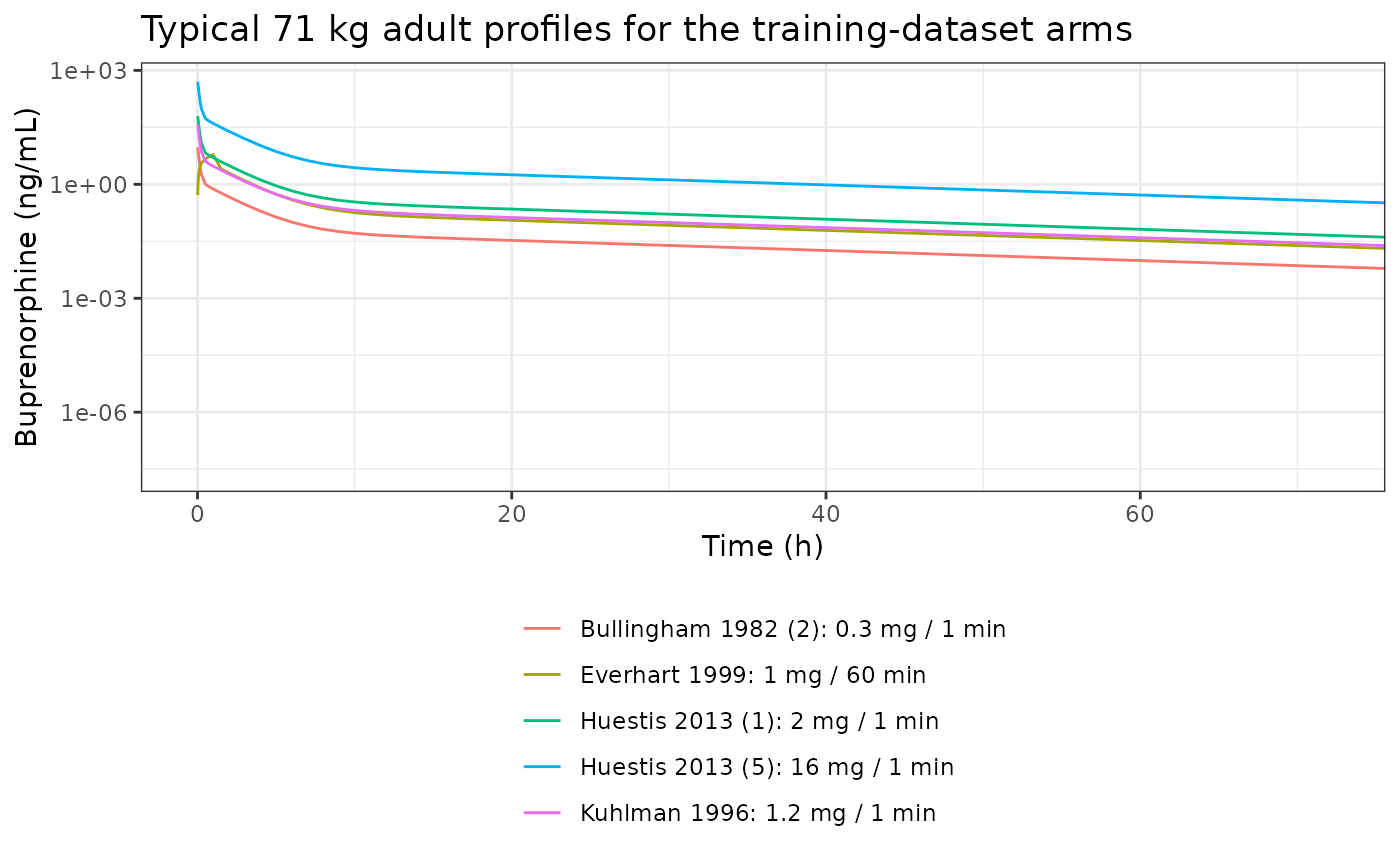
PKNCA validation
conc <- sim_adult |>
  filter(!is.na(Cc)) |>
  select(id, time, Cc, arm)
doses <- arms |>
  mutate(time = 0, amt = dose_mg * 1000) |>
  select(id, time, amt, arm)

o_conc <- PKNCA::PKNCAconc(conc, Cc ~ time | arm + id,
  concu = "ng/mL", timeu = "min")
o_dose <- PKNCA::PKNCAdose(doses, amt ~ time | arm + id, doseu = "ug")
intervals <- data.frame(start = 0, end = Inf, cmax = TRUE, tmax = TRUE,
  aucinf.obs = TRUE, half.life = TRUE)
nca <- PKNCA::pk.nca(PKNCA::PKNCAdata(o_conc, o_dose, intervals = intervals))

nca_wide <- as.data.frame(nca$result) |>
  select(arm, PPTESTCD, PPORRES) |>
  pivot_wider(names_from = PPTESTCD, values_from = PPORRES) |>
  left_join(arms, by = "arm") |>
  mutate(
    auc_closed_form = dose_mg * 1000 / cl,
    auc_pct_diff = 100 * (aucinf.obs / auc_closed_form - 1),
    half_life_h = half.life / 60
  )

nca_wide |>
  mutate(across(c(cmax, aucinf.obs, auc_closed_form, half_life_h), ~ signif(.x, 3)),
    auc_pct_diff = round(auc_pct_diff, 2)) |>
  select(arm, cmax, aucinf.obs, auc_closed_form, auc_pct_diff, half_life_h) |>
  dplyr::rename(
    "Arm" = arm, "Cmax (ng/mL)" = cmax,
    "AUC0-inf (ng*min/mL), PKNCA" = aucinf.obs,
    "Dose / CL (ng*min/mL)" = auc_closed_form,
    "AUC difference (%)" = auc_pct_diff, "t1/2 (h), PKNCA" = half_life_h
  ) |>
knitr::kable()| Arm | Cmax (ng/mL) | AUC0-inf (ng*min/mL), PKNCA | Dose / CL (ng*min/mL) | AUC difference (%) | t1/2 (h), PKNCA |
|---|---|---|---|---|---|
| Bullingham 1982 (2): 0.3 mg / 1 min | 9.4 | 308 | 305 | 0.71 | 22.6 |
| Everhart 1999: 1 mg / 60 min | 6.1 | 1040 | 1020 | 1.89 | 22.6 |
| Huestis 2013 (1): 2 mg / 1 min | 62.7 | 2050 | 2040 | 0.71 | 22.6 |
| Huestis 2013 (5): 16 mg / 1 min | 502.0 | 16400 | 16300 | 0.71 | 22.6 |
| Kuhlman 1996: 1.2 mg / 1 min | 37.6 | 1230 | 1220 | 0.71 | 22.6 |
stopifnot(
  # Trapezoidal AUC0-inf on a sampling grid against the exact Dose / CL.
  all(abs(nca_wide$auc_pct_diff) < 3),
  # The log-linear terminal fit recovers the terminal eigenvalue half-life.
  all(abs(nca_wide$half_life_h / half_lives_h[3] - 1) < 0.05)
)
The paper does not report compartmental NCA summaries for the three-compartment model, so the PKNCA block checks the simulation against the model’s own closed-form identities.
Preterm neonates: the two clearance exponents
The paper reports that the allometric model with the fixed exponent of 0.75 predicted the preterm-neonate concentrations poorly (mean relative deviation 12.46) and that the age-dependent exponent of 1.2 for clearance improved them (mean relative deviation 2.08; main text Section 3.3). The observed Cmax values of the 12 Barrett 1993 neonates (Supplementary Table S6, ‘Obs’ column) are compared below with the typical-value predictions under each exponent.
barrett <- tibble::tibble(
  id = 1:12,
  WT = c(1.5, 0.9, 1.3, 1.8, 1.5, 1.2, 1.1, 1.8, 1.6, 2.4, 1.6, 1.0),
  rate_ugkgh = c(0.72, 0.72, 0.72, 0.72, 0.72, 1.44, 1.44, 0.72, 2.16, 0.72,
    0.72, 0.72),
  dur_h = c(48, 24, 11, 42, 42, 23, 77, 42, 81, 43, 76, 118),
  cmax_obs = c(3.02, 2.80, 0.73, 2.29, 4.55, 3.20, 4.46, 4.17, 10.42, 2.50,
    3.33, 7.59)
)

ev_preterm <- bind_rows(lapply(seq_len(nrow(barrett)), function(i) {
  b <- barrett[i, ]
  t_end <- 30 + b$dur_h * 60
  bind_rows(
    # 3 ug/kg loading dose over 30 min (Table S2)
    tibble::tibble(id = b$id, time = 0, evid = 1, amt = 3 * b$WT,
      rate = 3 * b$WT / 30, cmt = "central"),
    # maintenance infusion, started at the end of the loading dose
    tibble::tibble(id = b$id, time = 30, evid = 1,
      amt = b$rate_ugkgh * b$WT * b$dur_h, rate = b$rate_ugkgh * b$WT / 60,
      cmt = "central"),
    tibble::tibble(id = b$id, time = sort(unique(c(seq(0, t_end + 12 * 60, by = 30), t_end))),
      evid = 0, amt = 0, rate = 0, cmt = "central")
  ) |>
    mutate(WT = b$WT)
}))

sim_preterm <- bind_rows(lapply(c(0.75, 1.2), function(e) {
  m <- mod |> rxode2::ini(e_wt_cl = e)
  rxode2::rxSolve(m, events = ev_preterm, returnType = "data.frame",
    keep = "WT") |>
    mutate(exponent = paste("CL exponent", e))
}))
#> ℹ change initial estimate of `e_wt_cl` to `0.75`
#> ℹ change initial estimate of `e_wt_cl` to `1.2`

cmax_cmp <- sim_preterm |>
  group_by(exponent, id) |>
  summarise(cmax_pred = max(Cc), .groups = "drop") |>
  left_join(barrett, by = "id") |>
  mutate(ratio = cmax_pred / cmax_obs)

gmfe <- cmax_cmp |>
  group_by(exponent) |>
  summarise(
    GMFE = exp(mean(abs(log(ratio)))),
    median_ratio = median(ratio),
    within_2fold = sum(ratio >= 0.5 & ratio <= 2),
    .groups = "drop"
  )
knitr::kable(gmfe, digits = 2,
caption = "Predicted versus observed Cmax in the 12 preterm neonates.")| exponent | GMFE | median_ratio | within_2fold |
|---|---|---|---|
| CL exponent 0.75 | 3.32 | 0.34 | 1 |
| CL exponent 1.2 | 2.00 | 0.51 | 7 |
ggplot(cmax_cmp, aes(cmax_obs, cmax_pred, colour = exponent)) +
  geom_point() +
  geom_abline(slope = 1) +
  geom_abline(slope = c(0.5, 2), linetype = 2) +
  scale_x_log10() +
  scale_y_log10() +
  labs(x = "Observed Cmax (ng/mL)", y = "Predicted Cmax (ng/mL)", colour = NULL,
    caption = "Compare with Figure 5d and Supplementary Figure S7 of Kovar 2020.") +
  theme_bw()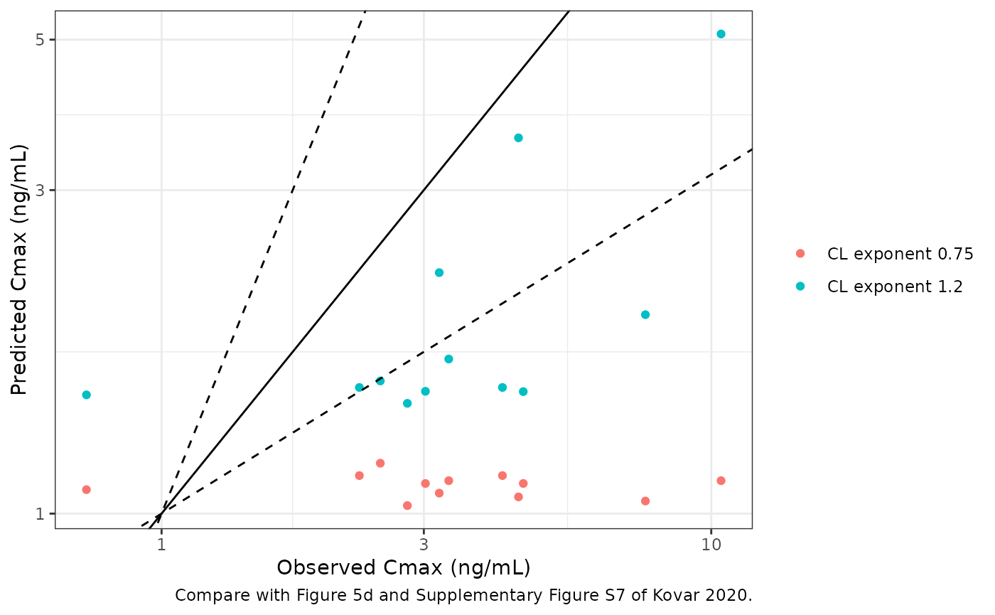
g075 <- gmfe$median_ratio[gmfe$exponent == "CL exponent 0.75"]
g12 <- gmfe$median_ratio[gmfe$exponent == "CL exponent 1.2"]
f075 <- gmfe$GMFE[gmfe$exponent == "CL exponent 0.75"]
f12 <- gmfe$GMFE[gmfe$exponent == "CL exponent 1.2"]
stopifnot(
  # Deterministic typical-value solves (no random effects), so these values
  # do not vary between machines.
  # Exponent 1.2: about 2-fold low, as the paper's MRD of 2.08 implies
  # (median ratio 0.51 when written).
  g12 > 0.35, g12 < 1.5,
  # Exponent 0.75: further low (median ratio 0.34 when written); the Cmax is
  # dominated by the 30-min loading dose into the small central volume, so the
  # 5.7-fold difference in clearance shows only partly in Cmax.
  g075 < 0.4,
  f12 < f075
)
Both variants underpredict the neonatal Cmax; the age-dependent exponent reduces the error, in line with the paper’s Discussion: the age-dependent exponent improved the allometric predictions in preterm neonates, while the PBPK scaling remained superior to allometry.
Children
ev_child <- rxode2::et(amt = 3 * 21.4, rate = 3 * 21.4 / 2, cmt = "central") |>
  rxode2::et(c(0, 2, 5, 10, 15, 30, 45, seq(60, 12 * 60, by = 30)),
    cmt = "central") |>
  as.data.frame() |>
  mutate(WT = 21.4)
sim_child <- rxode2::rxSolve(mod, events = ev_child, returnType = "data.frame",
  keep = "WT")
ggplot(sim_child[sim_child$time > 0, ], aes(time / 60, Cc)) +
  geom_line() +
  scale_y_log10() +
  labs(x = "Time (h)", y = "Buprenorphine (ng/mL)",
    title = "Typical 21.4 kg child, 3 ug/kg over 2 min (Olkkola 1989 regimen)",
    caption = "Compare with the allometric-scaling panels of Supplementary Section 4.2.") +
  theme_bw()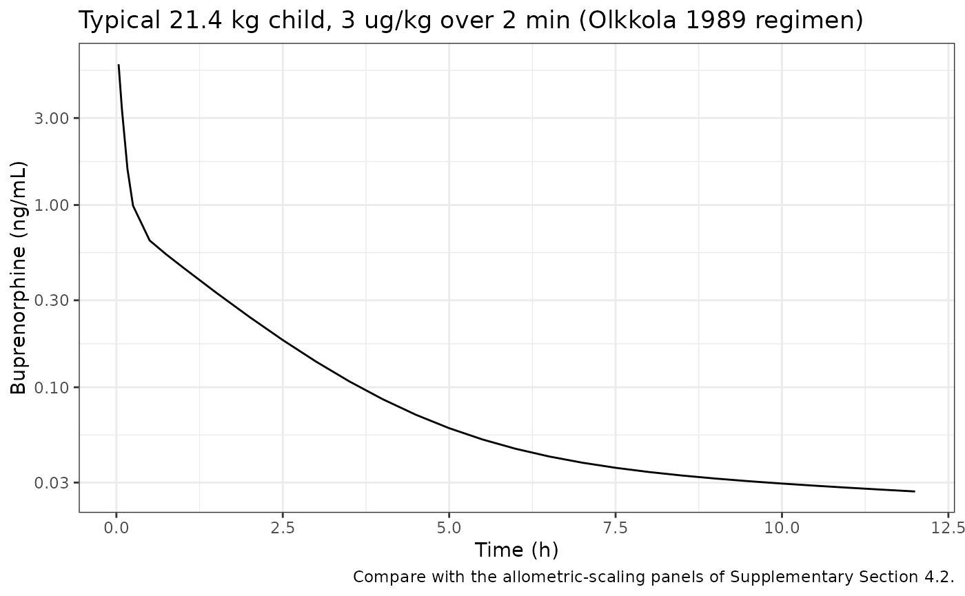
Assumptions and deviations
- Only the allometric comparator is packaged. The paper’s primary result is a PK-Sim whole-body PBPK model; it depends on software-database physiology and calculated partition coefficients that the publication does not print, so it is not reproduced here.
- No variability. The three-compartment model was fitted to digitised mean profiles, and no inter-individual or residual variability was reported, so the model carries typical values only and no residual error model.
-
Pooled sampling site. The training data mix
arterial (Bullingham) and venous (Everhart, Huestis, Kuhlman) samples;
Ccis therefore a pooled plasma concentration, not specifically arterial or venous. - Unit conversion. Table S4 gives clearances in mL/min; the model stores them in L/min (divided by 1000) so that time is in minutes, volumes in litres and concentrations in ng/mL for doses in ug.
-
Exponent variant. The age-dependent clearance
exponent of 1.2 (Equation S15) is not a separate model; set
e_wt_cl = 1.2viaini()to reproduce it, as done above for the preterm neonates. - Table S4 rounding slip. The children’s V2 is printed as 32.0 L; the printed scaling equations give 31.6 L at 21.4 kg, and the other cells of the same row agree with 21.4 kg. The model follows the equations.
- Barrett 1993 dosing timing. Table S2 gives a 30-min loading dose followed by the maintenance infusion; the maintenance infusion is assumed to start at the end of the loading dose.