Tacrolimus in chronic kidney disease (El-Khateeb 2023)
Source:vignettes/articles/ElKhateeb_2023_tacrolimus.Rmd
ElKhateeb_2023_tacrolimus.RmdModel and source
- Citation: El-Khateeb E, Chinnadurai R, Al Qassabi J, Scotcher D, Darwich AS, Kalra PA, Rostami-Hodjegan A. Using Prior Knowledge on Systems Through PBPK to Gain Further Insight into Routine Clinical Data on Trough Concentrations: The Case of Tacrolimus in Chronic Kidney Disease. Ther Drug Monit. 2023;45(6):743-753. doi:10.1097/FTD.0000000000001108. Structural equations are Eq. 3-17; the bottom-up formulas and system constants are those of the authors’ calculation spreadsheet (Supplementary File 1) and Monolix script (Supplementary File 2); estimates are the Table 1 ‘Base’ row.
- Description (base model): Middle-out (PBPK-informed) one-compartment population PK model for oral tacrolimus whole-blood trough concentrations in adult renal transplant recipients with chronic kidney disease (base model, no covariate on intrinsic clearance). The only estimated structural parameter is the hepatic unbound intrinsic clearance CLint; hepatic blood flow, the blood:plasma ratio, the unbound fraction, renal clearance (filtration only), bioavailability (fa * fg * fh, well-stirred liver) and the steady-state blood volume of distribution are computed bottom-up from body weight, height, sex, hematocrit, serum albumin and eGFR at every occasion. Absorption is taken as complete within a dosing interval (ka >> kel), so the dose enters the central compartment directly. Between-subject and inter-occasion variability on CLint, where every trough measurement is its own occasion. Sibling covariate models: ElKhateeb_2023_tacrolimus_egfr and ElKhateeb_2023_tacrolimus_ckdstage.
- Article: https://doi.org/10.1097/FTD.0000000000001108 (open access, PMC10635338)
El-Khateeb et al. combined a bottom-up (PBPK-style) description of
tacrolimus disposition with a top-down population fit of routine
therapeutic-drug-monitoring troughs. Everything except the hepatic
unbound intrinsic clearance CLint is computed from patient
data at every trough: hepatic blood flow from body weight, the
blood:plasma ratio from hematocrit, the unbound fraction from albumin,
renal clearance from eGFR, and the steady-state volume from a Rodgers
tissue composition. CLint was then estimated in Monolix
with between-subject and inter-occasion variability, and three covariate
models for kidney function on CLint were compared in
parallel against the base model (Supplementary File 3, Figure 2).
The library carries three of the four fits, one file each:
| Model | Covariate on CLint | Table 1 row | AIC |
|---|---|---|---|
ElKhateeb_2023_tacrolimus |
none (base model) | Base | 7297.1 |
ElKhateeb_2023_tacrolimus_egfr |
eGFR, continuous | eGFR | 7249.14 |
ElKhateeb_2023_tacrolimus_ckdstage |
CKD stage 1-5, categorical | CKD stage | 7264.74 |
The fourth, CKD group (stable vs failing transplant), was non-significant (beta = -0.0073, RSE 1880%) and is the base model in all but name, so it is not packaged.
Population
Forty adult renal transplant recipients from the Salford Royal Hospital transplant database (UK), 20 with stable graft function and 20 with failing graft function (annual eGFR fall above 5 mL/min/1.73 m^2), matched for age, sex and ethnicity. Median age 41.6 years (IQR 33.6-50.9), 57.5% male, 77.5% white; baseline eGFR median 45 mL/min/1.73 m^2 (IQR 34.5-55.5), hematocrit 0.36 (0.32-0.41) and albumin 43 g/L (40-45) (Results; Supplementary File 3 Table 2). All received immediate-release tacrolimus (Prograf) twice daily, 2-14 mg/day. The analysis used 1167 steady-state whole-blood troughs (median 29 per patient) over a median 3.3-year follow-up, during which eGFR ranged 4.97-119.2 mL/min/1.73 m^2 (CKD stages 1-5). Troughs were normalised to 5 mg every 12 h.
The same information is available programmatically via
readModelDb("ElKhateeb_2023_tacrolimus")()$population.
Source trace
Every ini() value carries an in-file comment pointing to
its source. The bottom-up formulas and constants come from the authors’
calculation spreadsheet (Supplementary File 1) and agree with the
printed equations; the structural closed form is the Monolix script
(Supplementary File 2).
| Equation / parameter | Value | Source location |
|---|---|---|
| Trough at steady state | Dose * F * exp(-kel*tau) / (Vss,b * (1 - exp(-kel*tau))) |
Eq. 3 and 17; Supplementary File 2 |
f(central) = F |
fa * (1 - egut) * (1 - CLh,b/Qh) |
Eq. 4-5 |
fa |
1 (fixed) | Methods below Eq. 5 |
egut |
0.86 (fixed; fg = 0.14) | Methods below Eq. 5 |
kel |
(CLr,b + CLh,b) / Vss,b |
Eq. 6 |
CLr,b |
fub * eGFR (L/h/1.73 m^2) |
Eq. 7 |
CLh,b |
Qh * fub * CLint / (Qh + fub * CLint) |
Eq. 8 (well-stirred liver) |
fub |
fup / (B/P) |
Eq. 9 |
fup |
1 / (1 + (ALB/45) * (1 - 0.013)/0.013) |
Eq. 10 |
Vss,b |
(Vp + Ve * E:P + 10 * sum(Vt * Pt:p)) / (B/P) |
Eq. 11; scaling factor 10 in Methods |
Vp, Ve
|
Vb * (1 - Hct), Vb * Hct
|
Eq. 12-13 |
Vb |
sex-specific in height (m) and weight | Eq. 14-15 |
B/P |
E:P * Hct + (1 - Hct), E:P = 77.27 |
Eq. 16; Supplementary File 1 |
| Organ masses, densities | ICRP female 60 kg / male 73 kg, scaled by WT | Supplementary File 1 |
Pt:p (13 tissues) |
0.52-1.91 | Supplementary File 3 Table 1 |
Qh |
0.227 * 187 * WT^0.81 mL/min |
Supplementary File 2 |
lclint |
log(5886.7) / log(4350.89) / log(6377.46) | Table 1 Base / eGFR / CKD stage |
e_crcl_clint |
0.11 per L/h/1.73 m^2 | Table 1 eGFR row (form: see Assumptions) |
e_ckd2_clint … e_ckd5_clint
|
-0.047, -0.011, -0.1, -0.19, -0.31 | Table 1 CKD stage rows (sign: see Assumptions) |
etalclint |
0.32^2 / 0.33^2 / 0.33^2 | Table 1 omega (Monolix SD) |
etaiov_lclint |
0.2^2 / 0.18^2 / 0.19^2 | Table 1 gamma (Monolix SD) |
propSd |
0.101 / 0.109 / 0.105 | Not reported; see Assumptions |
Bottom-up quantities
The model computes the authors’ per-trough regressors internally from
six covariates (WT, HT, SEXF,
HCT, ALB, CRCL). The virtual
cohort below draws them from the distributions of the 1167 measurements
in Supplementary File 1 (weight median 73 kg, log-SD 0.23; height median
173 cm in men and 160 cm in women; hematocrit mean 0.364, SD 0.055;
albumin mean 42.3 g/L, SD 4.9; eGFR median 38.6 mL/min/1.73 m^2, log-SD
0.51; about half the measurements from men).
set.seed(20231108)
rxode2::rxSetSeed(20231108)
n_sub <- 200
cohort <- tibble(
  id = seq_len(n_sub),
  SEXF = rbinom(n_sub, 1, 0.5),
  HT = ifelse(SEXF == 1, rnorm(n_sub, 160, 6), rnorm(n_sub, 173, 6)),
  WT = pmin(pmax(exp(rnorm(n_sub, log(73), 0.23)), 40), 141),
  HCT = 100 * pmin(pmax(rnorm(n_sub, 0.364, 0.055), 0.21), 0.59),
  ALB = pmin(pmax(rnorm(n_sub, 42.3, 4.9), 19), 53),
  CRCL = pmin(pmax(exp(rnorm(n_sub, log(38.6), 0.51)), 5), 119)
)

# The same formulas as model(), written out once so the vignette can check
# the model's internal quantities against the paper's summary numbers.
bottom_up <- function(d, kp_scale = 10, clint = 5886.7) {
  hct <- d$HCT / 100
  bpr <- 77.27 * hct + 1 - hct
  fup <- 1 / (1 + (d$ALB / 45) * (1 - 0.013) / 0.013)
  fub <- fup / bpr
  vb <- ifelse(d$SEXF == 1,
    0.3561 * (d$HT / 100)^3 + 0.03308 * d$WT + 0.1833,
    0.3669 * (d$HT / 100)^3 + 0.03219 * d$WT + 0.6041
  )
  mass_f <- c(22500, 7800, 1300, 1965, 250, 275, 1400, 420, 120, 17500, 2300, 130, 4040) / 60
  mass_m <- c(18200, 10500, 1450, 2110, 330, 310, 1800, 500, 140, 29000, 3300, 150, 5210) / 73
  dens <- c(950, 1920, 1050, 1040, 1050, 1050, 1070, 384, 1050, 1050, 1090, 1040, 1050)
  kp <- c(1.90, 1.89, 1.91, 1.56, 0.74, 0.96, 1.33, 0.52, 1.37, 0.96, 1.07, 0.97, 1.90)
  vtkp <- ifelse(d$SEXF == 1, sum(mass_f / dens * kp), sum(mass_m / dens * kp))
  vss_b <- (vb * (1 - hct) + vb * hct * 77.27 + kp_scale * d$WT * vtkp) / bpr
  qh <- 0.227 * 187 * d$WT^0.81 * 0.06
  clh <- qh * fub * clint / (qh + fub * clint)
  clr <- fub * d$CRCL * 0.06
  fbio <- 0.14 * (1 - clh / qh)
  kel <- (clh + clr) / vss_b
  tibble(bpr, fup, fub, vss_b, qh, clh, fbio, kel,
    trough = 5000 * fbio * exp(-kel * 12) / (vss_b * (1 - exp(-kel * 12)))
  )
}
bu <- bottom_up(cohort)
bu_unscaled <- bottom_up(cohort, kp_scale = 1)

checks <- tibble(
  Quantity = c(
    "Mean B/P", "Mean Vss,b before the x10 Pt:p scaling (L)",
    "Mean CLh,b at CLintpop of the base model (L/h)"
  ),
  Paper = c(28.8, 8.2, 2.84),
  Source = c("Results, B/P 19-46", "Methods, after Eq. 16", "Discussion (2.84 +/- 0.94)"),
  Simulated = c(mean(bu$bpr), mean(bu_unscaled$vss_b), mean(bu$clh))
)
knitr::kable(checks, digits = 2, caption = "Bottom-up quantities in the virtual cohort vs the paper.")| Quantity | Paper | Source | Simulated |
|---|---|---|---|
| Mean B/P | 28.80 | Results, B/P 19-46 | 29.29 |
| Mean Vss,b before the x10 Pt:p scaling (L) | 8.20 | Methods, after Eq. 16 | 8.17 |
| Mean CLh,b at CLintpop of the base model (L/h) | 2.84 | Discussion (2.84 +/- 0.94) | 2.76 |
stopifnot(
  # Each is a cohort mean of a smooth function of covariates whose spread the
  # cohort reproduces, so a wrong constant (E:P, a Pt:p, a density, the 0.227
  # hepatic fraction of cardiac output) moves it by far more than 10%.
  abs(mean(bu$bpr) / 28.8 - 1) < 0.10,
  abs(mean(bu_unscaled$vss_b) / 8.2 - 1) < 0.10,
  abs(mean(bu$clh) / 2.84 - 1) < 0.10
)
The ODE reproduces the closed form
The packaged model is a one-compartment ODE with the dose entering
the central compartment (absorption complete within the interval) and
f(central) equal to the bottom-up bioavailability. At
steady state on 5 mg every 12 h its end-of-interval concentration must
equal Eq. 17 for every subject.
mod_base <- readModelDb("ElKhateeb_2023_tacrolimus")

ev_cf <- cohort |>
  mutate(OCC = 1) |>
  tidyr::crossing(evid = c(1, 0)) |>
  mutate(
    time = ifelse(evid == 1, 0, 12), amt = ifelse(evid == 1, 5, 0),
    ss = ifelse(evid == 1, 1, 0), ii = ifelse(evid == 1, 12, 0), cmt = "central"
  ) |>
  arrange(id, time, desc(evid))
# Two occasion levels are needed for the nested IOV; the typical-value solve
# ignores them.
ev_cf$OCC[ev_cf$id %% 2 == 0] <- 2

sim_cf <- rxode2::rxSolve(rxode2::zeroRe(mod_base), ev_cf,
  rtol = 1e-10, atol = 1e-12, ssRtol = 1e-10, ssAtol = 1e-12, maxsteps = 1e6,
  returnType = "data.frame"
)
#> ℹ parameter labels from comments will be replaced by 'label()'
rel_err <- sim_cf$Cc / bu$trough - 1
max(abs(rel_err))
#> [1] 3.90084e-10
stopifnot(max(abs(rel_err)) < 1e-6)
Covariate effects on CLint
Figure 4 of the paper relates the individual CLint estimates to eGFR and CKD stage. The packaged covariate models give the typical CLint below; the paper’s per-stage means are averages of individual (empirical Bayes) estimates, so they carry the random effects and are compared only for direction and size.
mod_egfr <- readModelDb("ElKhateeb_2023_tacrolimus_egfr")
mod_ckd <- readModelDb("ElKhateeb_2023_tacrolimus_ckdstage")
th_egfr <- rxode2::rxode(mod_egfr)$theta
#> ℹ parameter labels from comments will be replaced by 'label()'
th_ckd <- rxode2::rxode(mod_ckd)$theta
#> ℹ parameter labels from comments will be replaced by 'label()'

clint_egfr <- function(egfr) exp(th_egfr[["lclint"]] + th_egfr[["e_crcl_clint"]] * egfr * 0.06)
stage_coef <- c(
  "1" = 0, "2" = th_ckd[["e_ckd2_clint"]], "3a" = th_ckd[["e_ckd3a_clint"]],
  "3b" = th_ckd[["e_ckd3b_clint"]], "4" = th_ckd[["e_ckd4_clint"]], "5" = th_ckd[["e_ckd5_clint"]]
)
stage_tab <- tibble(
  `CKD stage` = names(stage_coef),
  `Typical CLint, CKD-stage model (L/h)` = exp(th_ckd[["lclint"]] + stage_coef),
  `Mean individual CLint, paper (L/h)` = c(7483, 6639, 6410, 5944, 6039, 4754)
)
knitr::kable(stage_tab, digits = 0, caption = "CLint by CKD stage (paper values: Results, Figure 4A).")| CKD stage | Typical CLint, CKD-stage model (L/h) | Mean individual CLint, paper (L/h) |
|---|---|---|
| 1 | 6377 | 7483 |
| 2 | 6085 | 6639 |
| 3a | 6308 | 6410 |
| 3b | 5771 | 5944 |
| 4 | 5274 | 6039 |
| 5 | 4678 | 4754 |
ggplot(tibble(egfr = seq(5, 120, by = 1)), aes(egfr, clint_egfr(egfr))) +
  geom_line() +
  geom_point(
    data = tibble(egfr = c(100, 75, 52.5, 37.5, 22.5, 10), clint = stage_tab$`Typical CLint, CKD-stage model (L/h)`),
    aes(egfr, clint), colour = "firebrick"
  ) +
  labs(
    x = "eGFR (mL/min/1.73 m^2)", y = "Typical CLint (L/h)",
    caption = "Line: eGFR model. Points: CKD-stage model at mid-stage eGFR. Compare Figure 4A/4C of El-Khateeb 2023."
  )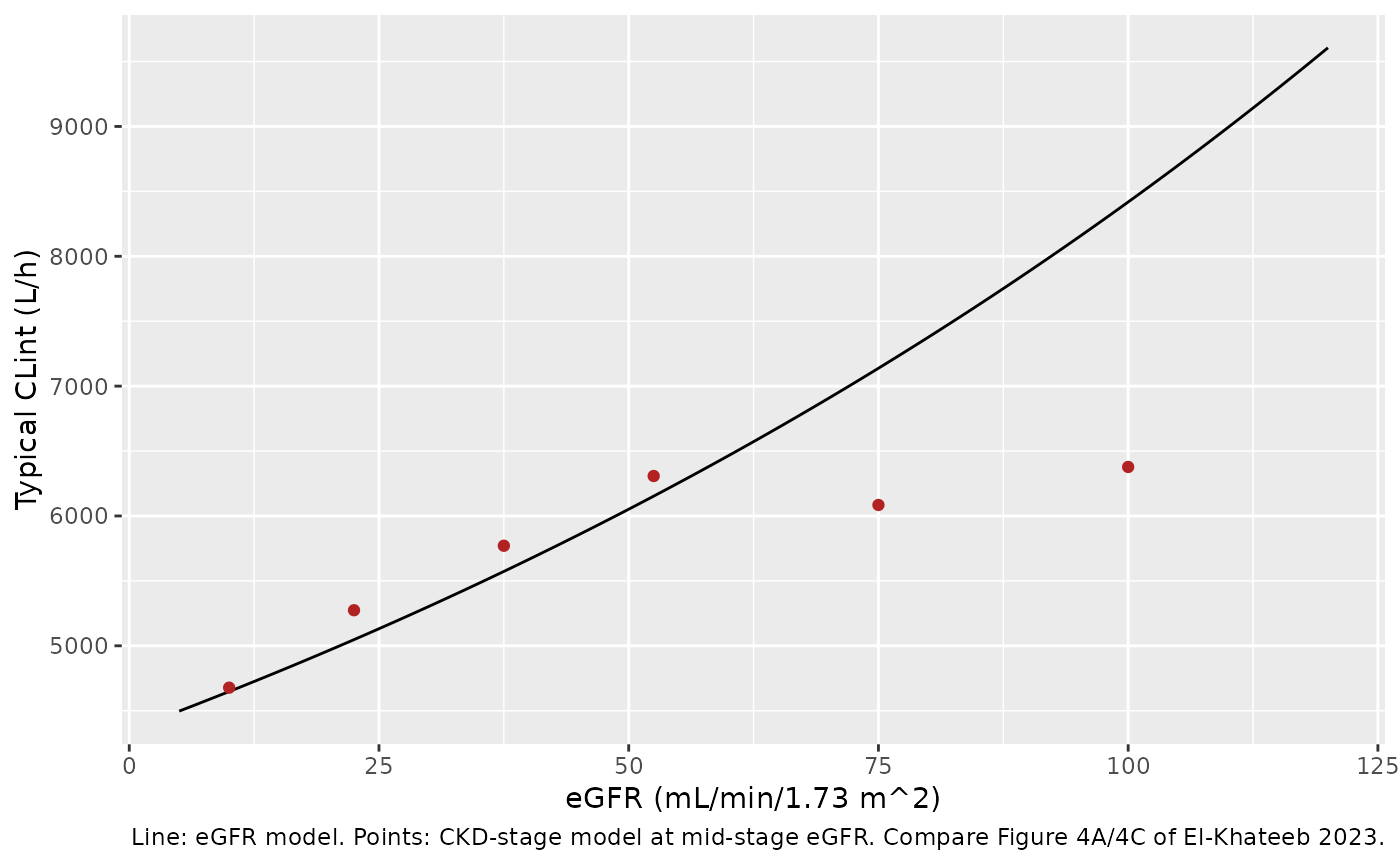
# Results: 'A 50% decrease in eGFR was associated with a 15% decrease in
# CLint'. Evaluated from the baseline median eGFR of 45 mL/min/1.73 m^2.
drop_half <- 1 - clint_egfr(45 / 2) / clint_egfr(45)
drop_half
#> [1] 0.138
# Results: 'CLint decreased by 36% in stage 5 CKD patients from stage 1'
# (individual means); the typical-value ratio of the stage model.
drop_stage5 <- 1 - exp(stage_coef[["5"]])
drop_stage5
#> [1] 0.266553
stopifnot(
  # The uncentred exponential gives 12-15% over the cohort's eGFR range; the
  # printed centred power form would give 7%.
  drop_half > 0.10, drop_half < 0.20,
  # Restored negative signs: stage 5 lower than stage 1.
  drop_stage5 > 0.2, drop_stage5 < 0.4,
  abs(stage_tab$`Typical CLint, CKD-stage model (L/h)`[6] / 4754 - 1) < 0.05
)
Dose-normalised trough VPC
Supplementary File 3 Figure 3 is the prediction-corrected VPC of the
base model: dose-adjusted troughs scatter around a median of about 13
ng/mL with a 95% band of roughly 6-30 ng/mL, flat over the follow-up.
The 1167 observed troughs in Supplementary File 1 have median 12.9
ng/mL, 2.5th percentile 3.9 and 97.5th percentile 39.8 ng/mL. The
simulation pools 1200 troughs: the covariates of the 200 virtual
subjects on each of six occasions, every one after steady-state dosing
at 5 mg every 12 h. Each subject-occasion is simulated as a virtual
subject of its own. With six steady-state records per subject in one
event table, switched through OCC, some of the later
troughs came back NA, so the troughs that share a set of covariates are
independent here; the pooled quantiles, which are what the table and the
assertions use, do not depend on that.
n_occ <- 6
# One steady-state record at time 0 and the trough 12 h later, per subject-occasion
# (id runs over n_sub * n_occ; OCC fixes the occasion's random effect).
ev_vpc <- cohort |>
  tidyr::crossing(OCC = seq_len(n_occ), evid = c(1, 0)) |>
  mutate(
    id = (OCC - 1L) * n_sub + id,
    time = ifelse(evid == 1, 0, 12),
    amt = ifelse(evid == 1, 5, 0), ss = ifelse(evid == 1, 1, 0),
    ii = ifelse(evid == 1, 12, 0), cmt = "central"
  ) |>
  arrange(id, time, desc(evid))

# rxode2 draws the occasion effect (`etaiov_lclint`) per subject and occasion only
# when some subject has two or more `OCC` levels. When every subject has exactly one,
# it treats `OCC` as a level above the subject and every subject on that occasion
# shares one draw. The extra record below (evid = 2: it doses and observes nothing)
# gives the first subject a second occasion level to select the per-subject draw.
ev_iov <- ev_vpc[ev_vpc$id == 1L & ev_vpc$evid == 0, ]
ev_iov$OCC <- n_occ + 1L
ev_iov$evid <- 2L
ev_iov$time <- 13
ev_vpc <- bind_rows(ev_vpc, ev_iov) |> arrange(id, time, desc(evid))

sim_vpc <- rxode2::rxSolve(mod_base, ev_vpc, maxsteps = 1e6, returnType = "data.frame")
#> ℹ parameter labels from comments will be replaced by 'label()'

# Every subject-occasion must have solved: an NA trough would otherwise leave the
# quantiles below without a trace.
troughs <- sim_vpc |> filter(time == 12)
stopifnot(nrow(troughs) == n_sub * n_occ, !anyNA(troughs$sim))
# One occasion effect per subject-occasion, not one per occasion: if rxode2's
# detection of the nesting changes, the render fails instead of sharing silently.
iov_per_occasion <- troughs |>
  group_by(OCC) |>
  summarise(n_distinct_iov = n_distinct(round(etaiov_lclint, 8)), .groups = "drop")
stopifnot(nrow(iov_per_occasion) == n_occ, all(iov_per_occasion$n_distinct_iov == n_sub))
# Follow-up day of the occasion, for the plot (occasions are 5000 h apart).
troughs$day <- ((troughs$OCC - 1) * 5000 + 12) / 24
#> Warning in Ops.factor(troughs$OCC, 1): '-' not meaningful for factors
vpc_tab <- tibble(
  Statistic = c("2.5th percentile", "Median", "97.5th percentile"),
  `Observed, Supplementary File 1 (ng/mL)` = c(3.9, 12.86, 39.77),
  `Simulated, base model (ng/mL)` = quantile(troughs$sim, c(0.025, 0.5, 0.975))
)
knitr::kable(vpc_tab, digits = 1, caption = "Dose-normalised troughs: simulated vs observed.")| Statistic | Observed, Supplementary File 1 (ng/mL) | Simulated, base model (ng/mL) |
|---|---|---|
| 2.5th percentile | 3.9 | 3.1 |
| Median | 12.9 | 13.1 |
| 97.5th percentile | 39.8 | 52.1 |
ggplot(troughs, aes(day, sim)) +
  geom_point(alpha = 0.15, colour = "darkgreen") +
  geom_hline(yintercept = quantile(troughs$sim, c(0.025, 0.5, 0.975)), linetype = c(2, 1, 2)) +
  scale_y_log10() +
  labs(
    x = "Time (days)", y = "Dose-adjusted trough (ng/mL)",
    caption = "Replicates the layout of Supplementary File 3 Figure 3 of El-Khateeb 2023 (base model)."
  )
#> Warning: Removed 1200 rows containing missing values or values outside the scale range
#> (`geom_point()`).
stopifnot(
  # Centre: a wrong CLint, volume or bioavailability term moves the median
  # by tens of percent.
  abs(median(troughs$sim) / 12.86 - 1) < 0.20,
  # Envelope, on robust quantiles of 1200 simulated troughs.
  quantile(troughs$sim, 0.975) > 25, quantile(troughs$sim, 0.975) < 60,
  quantile(troughs$sim, 0.025) > 2, quantile(troughs$sim, 0.025) < 7
)
PKNCA: steady-state interval by CKD stage
The paper reports no NCA. The steady-state dosing interval of a
typical patient in each CKD stage (CKD-stage model, median covariates,
eGFR at mid-stage) is summarised with PKNCA; cmin must
equal the closed-form trough and auclast must equal
F * Dose / CL for the interval.
typ <- tibble(
  treatment = c("1", "2", "3a", "3b", "4", "5"),
  CRCL = c(100, 75, 52.5, 37.5, 22.5, 10),
  id = seq_along(CRCL), SEXF = 0, HT = 173, WT = 73, HCT = 36, ALB = 43
)
grid <- seq(0, 12, by = 0.25)
ev_nca <- bind_rows(
  typ |> mutate(time = 0, evid = 1, amt = 5, ss = 1, ii = 12),
  typ |> tidyr::crossing(time = grid) |> mutate(evid = 0, amt = 0, ss = 0, ii = 0)
) |>
  mutate(cmt = "central", OCC = ifelse(id %% 2 == 0, 2, 1)) |>
  arrange(id, time, desc(evid))

sim_nca <- rxode2::rxSolve(rxode2::zeroRe(mod_ckd), ev_nca,
  rtol = 1e-10, atol = 1e-12, ssRtol = 1e-10, ssAtol = 1e-12, maxsteps = 1e6,
  keep = "treatment", returnType = "data.frame"
)
#> ℹ parameter labels from comments will be replaced by 'label()'

conc_df <- sim_nca |>
  filter(!is.na(Cc)) |>
  select(id, time, Cc, treatment)
dose_df <- ev_nca |>
  filter(evid == 1) |>
  select(id, time, amt, treatment)

conc_obj <- PKNCA::PKNCAconc(conc_df, Cc ~ time | treatment + id)
dose_obj <- PKNCA::PKNCAdose(dose_df, amt ~ time | treatment + id)
intervals <- data.frame(start = 0, end = 12, cmax = TRUE, cmin = TRUE, auclast = TRUE)
nca_res <- PKNCA::pk.nca(PKNCA::PKNCAdata(conc_obj, dose_obj, intervals = intervals))

nca_wide <- as.data.frame(nca_res) |>
  select(treatment, PPTESTCD, PPORRES) |>
  tidyr::pivot_wider(names_from = PPTESTCD, values_from = PPORRES)

# Closed-form references at the typical CLint of each stage.
ref <- typ |>
  mutate(clint = exp(th_ckd[["lclint"]] + stage_coef[treatment]))
ref_bu <- bind_cols(ref, bottom_up(ref, clint = ref$clint) |> select(-qh))
ref_bu <- ref_bu |>
  mutate(
    cmin_ref = trough,
    auc_ref = 1000 * 5 * fbio / (kel * vss_b)
  )
nca_cmp <- nca_wide |>
  left_join(ref_bu |> select(treatment, cmin_ref, auc_ref), by = "treatment")

nca_cmp |>
  dplyr::rename(
    "CKD stage" = treatment,
    "Cmax (ng/mL)" = cmax,
    "Cmin (ng/mL)" = cmin,
    "AUC0-12 (ng*h/mL)" = auclast,
    "Closed-form trough (ng/mL)" = cmin_ref,
    "F * Dose / CL (ng*h/mL)" = auc_ref
  ) |>
knitr::kable(digits = 2, caption = "Steady-state interval, typical patient by CKD stage (5 mg every 12 h).")| CKD stage | AUC0-12 (ng*h/mL) | Cmax (ng/mL) | Cmin (ng/mL) | Closed-form trough (ng/mL) | F * Dose / CL (ng*h/mL) |
|---|---|---|---|---|---|
| 1 | 229.51 | 29.24 | 11.66 | 11.66 | 229.51 |
| 2 | 240.60 | 30.12 | 12.52 | 12.52 | 240.60 |
| 3a | 232.15 | 29.45 | 11.87 | 11.87 | 232.15 |
| 3b | 253.79 | 31.18 | 13.54 | 13.54 | 253.79 |
| 4 | 277.73 | 33.10 | 15.42 | 15.42 | 277.73 |
| 5 | 313.18 | 35.97 | 18.22 | 18.22 | 313.18 |
Assumptions and deviations
-
Residual-error magnitude is not published. The
paper names the selected residual model (“proportional”) but reports no
value for it in Table 1, Supplementary File 3 Table 3 or anywhere else.
The maintainers estimated it by profile likelihood on the authors’ own
per-measurement dataset (Supplementary File 1), holding CLintpop, omega
and gamma at each model’s Table 1 values and integrating the
between-subject and per-trough inter-occasion effects by quadrature.
Giving that dataset to the model reproduces the published fit closely:
with the profiled value the marginal -2LL of the base model is 7266
against the published 7289.1, and freeing omega and gamma as well
returns 0.31 and 0.21 against the published 0.32 and 0.20. The resulting
propSd(0.101 base, 0.109 eGFR, 0.105 CKD stage) is extractor-derived, not a published estimate. -
Error model form. The paper states that
“observations were assumed to follow a log-normal distribution”, which
in Monolix makes the “proportional” error model proportional on the
log-transformed prediction. The model encodes that as
Cc ~ lnorm(NA) + propT(propSd). On the authors’ dataset this form fits about 45 -2LL units better than a proportional error on the untransformed scale, and its freely estimated omega and gamma (0.31, 0.21) sit closer to the published values than those of the untransformed form (0.31, 0.25). -
eGFR covariate form. Eq. 19 prints a power model
centred at the median eGFR,
(eGFR/median)^beta. With beta = 0.11 that form changes CLint by less than 10% across the cohort, which leaves CLintpop = 4350.89 L/h 26% below the base model everywhere and contradicts both the reported likelihood gain and the Results statement that halving eGFR lowers CLint by 15%. Monolix’s default for a continuous covariate on a log-normal parameter, the uncentredexp(beta * eGFR)with eGFR in L/h/1.73 m^2 (the unit of the script’s regressor), reproduces all three: typical CLint 5600 L/h at the median eGFR, a 12-15% fall per halving, and a -2LL drop of 55 from the base model on the authors’ dataset against the published 50 (the centred power form drops it by 2). The model uses the uncentred exponential. - CKD-stage coefficient signs. Table 1 prints the stage coefficients without signs. Read as positive in Eq. 20 they would raise CLint with advancing CKD, the opposite of the paper’s conclusion. The model uses them as negative; the stage-5 typical CLint, 4677 L/h, then matches the reported stage-5 mean of 4754 L/h, and on the authors’ dataset the negative set lowers -2LL by 45 from the base model (published 42) while the positive set raises it by 160.
- CKD stage is derived from eGFR inside the model with the thresholds of the authors’ spreadsheet (90, 60, 45, 30, 15 mL/min/1.73 m^2), which is how the stage column of Supplementary File 1 was computed per measurement.
- E:P = 77.27, the value the authors’ spreadsheet uses to compute every blood:plasma ratio in the fitted dataset; the text quotes the fit as 77.4.
- eGFR enters renal clearance unadjusted for body surface area (L/h/1.73 m^2 used as L/h), as in the Monolix script. Renal clearance is below 0.1% of total tacrolimus clearance, so this has no practical effect.
-
Absorption. The paper simplifies its
first-order-absorption trough equation by assuming absorption is
complete within the dosing interval and never estimates ka, so the dose
enters
centraldirectly withf(central)equal to the bottom-up bioavailability. Concentrations within the interval (in particular Cmax) are therefore those of an instantaneous input and should not be read as predictions of the real oral peak; the model is built for troughs. -
Inter-occasion variability uses the native nested
random effect
etaiov_lclint ~ ... | OCC, with one occasion per trough as in the paper. Event tables must carry anOCCcolumn, and rxode2 draws the occasion effect per subject and occasion only when some subject has at least two occasions; when every subject has exactly one, all subjects on the same occasion share one draw. The VPC event table therefore adds one record that gives one subject a second occasion, and asserts the number of distinct occasion effects. The library’s convention checker reportsOCCas a covariate not referenced inmodel(), because it is consumed by theini()nesting syntax. - Virtual cohort. Height and weight are not tabulated in the article; the cohort’s covariate distributions are summaries of the per-measurement spreadsheet (Supplementary File 1), and covariates are held constant within each virtual subject. The covariates are drawn independently of one another, so the cohort lacks the correlations of the real patients, which is one reason the simulated 97.5th percentile of the dose-normalised trough (about 45-50 ng/mL) runs above the observed 39.8 ng/mL while the median matches.
- No erratum or correction notice for this article was found in Europe PMC (no linked correction on PMID 37315152; checked 2026-10-28).