Moxifloxacin (Willmann 2019)
Source:vignettes/articles/Willmann_2019_moxifloxacin.Rmd
Willmann_2019_moxifloxacin.RmdModel and source
- Citation: Willmann S, Frei M, Sutter G, Coboeken K, Wendl T, Eissing T, Lippert J, Stass H (2019). Application of physiologically-based and population pharmacokinetic modeling for dose finding and confirmation during the pediatric development of moxifloxacin. CPT: Pharmacometrics & Systems Pharmacology 8(9):654-663. doi:10.1002/psp4.12446. Final parameter estimates are from Supplementary Table S2 (final population PK model O6/run021); the model structure, the a-priori allometric exponents, the logit bioavailability parameterization, the zero-fixed absorption-rate and bioavailability etas and the three-way residual-error stratification are from the NONMEM control stream reproduced verbatim in Supplementary Material S1 (Model Code).
- Description: Three-compartment population PK model for moxifloxacin in children and adolescents aged 3 months to <18 years (Willmann 2019), with first-order absorption from an oral depot, logit-scale absolute bioavailability, and a-priori (not estimated) allometric body-weight scaling of all clearance and volume parameters with the canonical exponents 0.75 and 1.0. The structural parameters are reported per-kg (CL, Q in L/h/kg^0.75; V in L/kg) rather than normalized to a reference weight, so no centering weight enters the model. Interindividual variability was retained on CL and on the central volume only; the source held the absorption-rate and bioavailability etas at zero. Residual variability is proportional with three separate magnitudes, selected by development phase and route: phase I intravenous, phase III intravenous and phase III oral. The covariate screen (age, serum creatinine, estimated glomerular filtration rate, study and sex) retained nothing beyond the a-priori weight scaling. The companion whole-body PBPK model of the same paper is a PK-Sim / MoBi platform model whose physiological parameters come from the vendor’s internal databases and are not printed in the paper; it is therefore not reproducible as an rxode2 model and is not encoded here.
- Article: https://doi.org/10.1002/psp4.12446
- Supplement (Supplementary Methods, Tables S1-S2, Figures S1-S6):
PSP4-8-654-s001.pdf, published with the open-access article (PMC6765696). - Supplement (final NONMEM control stream, run
O6/run021):PSP4-8-654-s002.txt, same archive.
Willmann 2019 is a “learn and confirm” case study that carries two distinct models. The learning step is a whole-body PBPK model for moxifloxacin and its two metabolites, built in PK-Sim and MoBi and scaled from adults to children; the confirmation step is the pediatric population PK model fitted in NONMEM to the pooled phase I and phase III data. Only the popPK model is packaged here – see Assumptions and deviations for why the PBPK layer is not reproducible from the material available when this model was built.
Population
The model was fitted to 186 pediatric subjects contributing 1,562 moxifloxacin plasma concentrations, pooled from two trials: a phase I single-dose intravenous study (study 11826, N = 31) and a phase III study in complicated intra-abdominal infection (study 11643, N = 451 randomized, 301 exposed to moxifloxacin, 155 contributing PK samples), covering 3 months to <18 years of age. During model development 33 concentrations were excluded as influential outliers and 14 concentrations from 12 subjects were retained as non-influential outliers. Twenty-eight phase III subjects switched from intravenous to oral treatment.
Young children were markedly underrepresented: only 11 subjects younger than 3 years contributed PK information (10 from phase I and 1 from phase III), i.e. 5.9% of the study population – which the authors flag as the main limit on the conclusions that can be drawn at the young end of the age range. The paper does not tabulate baseline weight, sex or race distributions.
The same information is available programmatically via the model’s
population metadata:
str(readModelDb("Willmann_2019_moxifloxacin")()$population)
#> List of 7
#>  $ species      : chr "human"
#>  $ n_subjects   : num 186
#>  $ n_studies    : num 2
#>  $ age_range    : chr "3 months to <18 years"
#>  $ disease_state: chr "Phase III: complicated intra-abdominal infection. Phase I: pediatric patients receiving a single intravenous dose."
#>  $ dose_range   : chr "Phase I: single intravenous dose 5-10 mg/kg. Phase III: multiple intravenous doses followed by oral doses -- 40"| __truncated__
#>  $ notes        : chr "186 pediatric subjects contributing 1,562 moxifloxacin plasma concentrations were available for model developme"| __truncated__
Source trace
Every ini() entry in
inst/modeldb/specificDrugs/Willmann_2019_moxifloxacin.R
carries an in-file comment naming its origin. They are collected here
for review. “Table S2” refers to the supplementary parameter table of
the final model O6/run021; “control stream” refers to the
NONMEM code in Supplementary Material S1
(PSP4-8-654-s002.txt).
| Equation / parameter | Value | Source location |
|---|---|---|
lka |
log(0.537) |
Table S2 TKA = 0.537 1/h (RSE 26.6%) |
lcl |
log(0.45) |
Table S2 TCL = 0.45 L/h/kg^0.75 (RSE 2.56%) |
lvc |
log(0.906) |
Table S2 TV2 = 0.906 L/kg (RSE 5.61%) |
lq |
log(1.74) |
Table S2 TQ3 = 1.74 L/h/kg^0.75 (RSE 15.1%) |
lvp |
log(0.732) |
Table S2 TV3 = 0.732 L/kg (RSE 6.15%) |
lq2 |
log(0.0889) |
Table S2 TQ4 = 0.0889 L/h/kg^0.75 (RSE 13.6%) |
lvp2 |
log(0.615) |
Table S2 TV4 = 0.615 L/kg (RSE 16.0%) |
logitfdepot |
log(0.866 / 0.134) |
Table S2 TF = 0.866 (RSE 4.26%); logit form from the
control stream $PK block |
e_wt_cl_q_q2 |
fixed(0.75) |
Methods “Pediatric popPK model”; control stream
WGHT**0.75 on TCL, TQ3,
TQ4
|
e_wt_vc_vp_vp2 |
fixed(1) |
Methods “Pediatric popPK model”; control stream WGHT on
TV2, TV3, TV4
|
etalcl |
0.113 |
Table S2 CL omega^2 = 0.113, CV 34.6%, eta-shrinkage 4.43% |
etalvc |
0.257 |
Table S2 V2 omega^2 = 0.257, CV 54.1%, eta-shrinkage 16.5% |
propSdPh1Iv |
sqrt(0.0233) |
Table S2 “11826, IV” sigma^2 = 0.0233, CV 15.3% |
propSdPh3Iv |
sqrt(0.114) |
Table S2 “11643, IV” sigma^2 = 0.114, CV 33.8% |
propSdPh3Oral |
sqrt(0.226) |
Table S2 “11643, PO” sigma^2 = 0.226, CV 47.5% |
| Three-compartment ODE system with first-order absorption | n/a | Control stream $SUBROUTINE ADVAN12 TRANS4; Results
“PopPK model in children” |
Absorption lag ALAG1 fixed at 0 (structurally
absent) |
n/a | Control stream $THETA entry 6, 0 FIX; not
listed in Table S2 |
IIV on ka and on F fixed at 0
(omitted) |
n/a | Control stream $OMEGA entries 1 and 4,
0.0 FIX
|
| Residual error branching by study then route | n/a | Control stream $ERROR block
(IF(STUD.EQ.11826), IF(ROUT.EQ.1)) |
Note that the structural typical values are per
kilogram (L/h/kg^0.75 for the clearances,
L/kg for the volumes). The control stream writes the
allometry as TCL = THETA(2)*WGHT**0.75 and
TV2 = THETA(3)*WGHT, with no reference weight, so no
centering constant enters the model. As a sanity check on the scale, the
model’s typical 70 kg adult clearance is 0.45 * 70^0.75 =
10.9 L/h and typical adult steady-state volume is
(0.906 + 0.732 + 0.615) * 70 = 158 L, both consistent with
the published adult moxifloxacin disposition the pediatric model was
scaled from.
Virtual cohort
The original data are not public. The cohort below reproduces the composition of the phase III intravenous population that Willmann 2019 Table 1 reports: four dose bands with exactly the subject counts of that table (83, 52, 7 and 1 subject, totalling 143), so the simulated attainment percentages are computed over the same denominators as the published ones. Every band is well under the 200-participants-per-arm cap.
Weight is the only covariate the model reads structurally. The paper does not tabulate weights, so within each band age is drawn uniformly over the band’s age window and weight comes from a piecewise-linear interpolation of the CDC 2000 sex-averaged 50th-percentile weight-for-age curve with lognormal scatter, with draws falling outside the band’s own weight limits rejected and redrawn rather than clamped onto the boundary. This reference curve is cohort-construction input only – it is not a model parameter and is not taken from Willmann 2019.
# rxSetSeed fixes rxode2's RNG per solver thread, not across thread counts, so
# CI draws a different cohort than a workstation does. Every assertion below is
# written so that it holds for any cohort this model can produce.
rxode2::rxSetSeed(20190915)
set.seed(20190915)

cdc_age_yr <- c(c(1, 2, 3, 4, 6, 9, 12, 18, 24) / 12, 3:18)
cdc_wt_kg <- c(
  4.4, 5.5, 6.3, 7.0, 7.9, 9.0, 9.9, 11.3, 12.5,
  14.3, 16.3, 18.3, 20.7, 23.2, 26.0, 29.2, 32.7,
  36.7, 41.3, 46.0, 50.6, 54.6, 58.0, 60.6, 62.6
)
cdc_weight_for_age <- function(age_yr) {
  stats::approx(cdc_age_yr, cdc_wt_kg, xout = age_yr, rule = 2)$y
}

# The four phase III intravenous dose bands of Willmann 2019 Table 1. `n_iv`
# and `n_po` are that table's subject counts for the AUC(0-24 h) rows.
# `mg_per_kg` is NA for the flat 400 mg band. Age windows are those the table
# attaches to each band; weight limits are the band's own.
bands <- tibble::tribble(
  ~band,                            ~age_lo, ~age_hi, ~wt_lo, ~wt_hi, ~mg_per_kg, ~flat_mg, ~tau, ~n_iv, ~n_po,
  "12 to <18 y, >=45 kg",              12,      18,     45,     95,         NA,      400,    24,    83L,   21L,
  "12 to <18 y <45 kg; 6 to <12 y",     6,      18,      8,     45,          4,       NA,    12,    52L,    6L,
  "2 to <6 y",                          2,       6,      0,    Inf,          5,       NA,    12,     7L,    1L,
  "3 months to <2 y",                0.25,       2,      0,    Inf,          6,       NA,    12,     1L,    0L
)
# Ordered factor so tables and facets follow the paper's row order.
band_levels <- bands$band

# Ten days of dosing, then AUC(0-24 h) and Cmax over the final 24 h. The
# slowest disposition rate constant of the three-compartment system scales as
# WT^-0.25, so the loading period is sized from the low-clearance tail of the
# 34.6% CV IIV rather than from the typical half-life; the steady-state check
# below verifies it was long enough for every simulated subject.
t_end <- 240
ss_start <- 216
ss_prev <- 192
infusion_h <- 1 # see Assumptions and deviations

obs_times <- sort(unique(c(
  seq(0, 24, by = 0.5), # first-day profile, for the figure
  seq(ss_prev, ss_start, by = 0.25), # previous interval, for the steady-state check
  seq(ss_start, t_end, by = 0.25) # the AUC(0-24 h) interval itself
)))

make_band <- function(row, n, route, id_offset) {
  if (n == 0L) {
    return(NULL)
  }
  # Weight limits are part of the band DEFINITION, not a clipping rule: a
  # 14-year-old weighing 50 kg belongs to the 400 mg once-daily band, not to
  # the 4 mg/kg band clamped down to 45 kg. Clamping would pile probability
  # mass onto the boundary and skew the band's exposure distribution, so
  # out-of-band draws are rejected and redrawn instead.
  draw <- function(k) {
    a <- stats::runif(k, row$age_lo, row$age_hi)
    list(age = a, wt = cdc_weight_for_age(a) * exp(stats::rnorm(k, 0, 0.13)))
  }
  age_yr <- numeric(0)
  wt <- numeric(0)
  for (attempt in seq_len(200)) {
    d <- draw(4L * n)
    ok <- d$wt >= row$wt_lo & d$wt <= row$wt_hi
    age_yr <- c(age_yr, d$age[ok])
    wt <- c(wt, d$wt[ok])
    if (length(wt) >= n) break
  }
  stopifnot(length(wt) >= n)
  age_yr <- age_yr[seq_len(n)]
  wt <- wt[seq_len(n)]
  amt <- if (is.na(row$mg_per_kg)) rep(row$flat_mg, n) else row$mg_per_kg * wt
  dose_times <- seq(0, t_end - row$tau, by = row$tau)
  # Scalars resolved here: `route` also exists as a column on the expanded
  # grid below, where dplyr would mask the function argument with it.
  is_iv <- identical(route, "IV")
  dose_cmt <- if (is_iv) "central" else "depot"

  subj <- tibble::tibble(
    id = id_offset + seq_len(n),
    band = row$band,
    route = route,
    WT = wt,
    AGE = age_yr,
    amt_mg = amt
  )

  doses <- tidyr::expand_grid(subj, time = dose_times) |>
    dplyr::mutate(
      evid = 1,
      amt = amt_mg,
      cmt = dose_cmt,
      # An IV dose with an explicit positive `rate` is a zero-order infusion of
      # duration amt/rate; oral doses enter the depot as a bolus (rate = 0).
      rate = if (is_iv) amt_mg / infusion_h else 0
    )

  obs <- tidyr::expand_grid(subj, time = obs_times) |>
    dplyr::mutate(evid = 0, amt = 0, cmt = "central", rate = 0)

  dplyr::bind_rows(doses, obs) |>
    dplyr::mutate(
      # Both covariates are read by the residual-error model only. The
      # simulated cohort is the phase III study, and the route flag follows
      # the arm being simulated.
      STUDY_PHASE3 = 1,
      ROUTE_ORAL = as.integer(!is_iv)
    ) |>
    dplyr::select(-amt_mg) |>
    dplyr::arrange(id, time, dplyr::desc(evid))
}

events_iv <- dplyr::bind_rows(lapply(seq_len(nrow(bands)), function(i) {
  make_band(bands[i, ], bands$n_iv[i], "IV", id_offset = 1000L * i)
}))
events_po <- dplyr::bind_rows(lapply(seq_len(nrow(bands)), function(i) {
  make_band(bands[i, ], bands$n_po[i], "PO", id_offset = 5000L + 1000L * i)
}))

stopifnot(
  dplyr::n_distinct(events_iv$id) == sum(bands$n_iv),
  dplyr::n_distinct(events_po$id) == sum(bands$n_po),
  !anyDuplicated(unique(events_iv[, c("id", "time", "evid")])),
  length(intersect(events_iv$id, events_po$id)) == 0
)
Simulation
mod <- readModelDb("Willmann_2019_moxifloxacin")

sim_iv <- rxode2::rxSolve(
  mod,
  events = as.data.frame(events_iv),
  keep = c("band", "route", "WT", "AGE")
) |>
  as.data.frame() |>
  dplyr::mutate(band = factor(band, levels = band_levels))
#> ℹ parameter labels from comments will be replaced by 'label()'

sim_po <- rxode2::rxSolve(
  mod,
  events = as.data.frame(events_po),
  keep = c("band", "route", "WT", "AGE")
) |>
  as.data.frame() |>
  dplyr::mutate(band = factor(band, levels = band_levels))

stopifnot(
  nrow(sim_iv) > 0, nrow(sim_po) > 0,
  all(is.finite(sim_iv$Cc)), all(sim_iv$Cc >= 0)
)
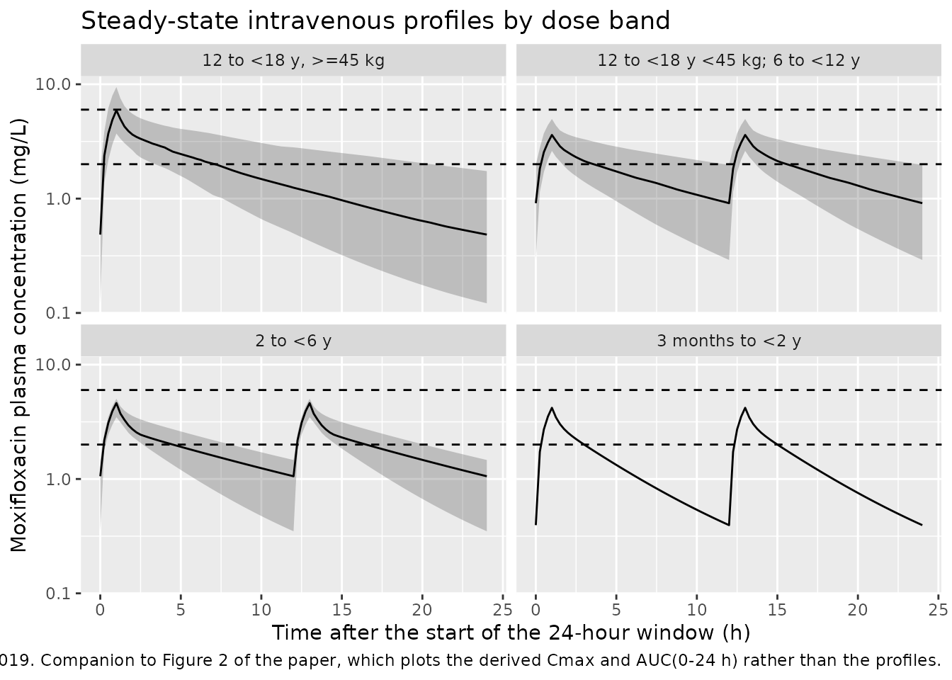
Willmann 2019 Table 1 and Figure 2 report AUC and Cmax “estimated
from the final popPK model”, i.e. individual model predictions carrying
each subject’s random effects but no residual error. Cc is
exactly that quantity, so it is the right column to run NCA on.
Structural gate: the steady-state mass balance
For any linear disposition model at steady state the AUC over one
24-hour window is pinned by clearance alone:
CL * AUC(0-24 h) must equal the amount actually reaching
the systemic circulation over those 24 hours. For the intravenous arm
that is the full daily dose; for the oral arm it is the daily dose
multiplied by the absolute bioavailability F. The check
below appends an AUC accumulator state to the model so the integral is
exact rather than trapezoidal, and runs it with the random effects
zeroed so the identity is deterministic.
mod_auc <- mod |>
  rxode2::zeroRe() |>
  rxode2::model(d/dt(aucCc) <- Cc, append = TRUE)
#> ℹ parameter labels from comments will be replaced by 'label()'
#> Warning: No sigma parameters in the model

gate_weights <- c(6, 12, 20, 35, 60, 90)

gate_events <- function(route, tau, mg_per_kg = NULL, flat_mg = NULL) {
  dplyr::bind_rows(lapply(seq_along(gate_weights), function(i) {
    wt <- gate_weights[i]
    amt <- if (is.null(flat_mg)) mg_per_kg * wt else flat_mg
    dose_times <- seq(0, t_end - tau, by = tau)
    dplyr::bind_rows(
      tibble::tibble(
        id = i, time = dose_times, evid = 1, amt = amt,
        cmt = if (route == "IV") "central" else "depot",
        rate = if (route == "IV") amt / infusion_h else 0
      ),
      tibble::tibble(
        id = i, time = c(ss_start, t_end), evid = 0, amt = 0,
        cmt = "central", rate = 0
      )
    ) |>
      dplyr::mutate(WT = wt, STUDY_PHASE3 = 1, ROUTE_ORAL = as.integer(route == "PO")) |>
      dplyr::arrange(id, time, dplyr::desc(evid))
  }))
}

mass_balance <- function(route, tau, mg_per_kg = NULL, flat_mg = NULL) {
  ev <- gate_events(route, tau, mg_per_kg, flat_mg)
  s <- as.data.frame(rxode2::rxSolve(mod_auc, events = as.data.frame(ev), keep = "WT"))
  daily <- ev |>
    dplyr::filter(evid == 1, time >= ss_start, time < t_end) |>
    dplyr::group_by(id) |>
    dplyr::summarise(daily_mg = sum(amt), .groups = "drop")
  s |>
    dplyr::filter(time %in% c(ss_start, t_end)) |>
    dplyr::group_by(id, WT, cl) |>
    dplyr::summarise(auc = diff(aucCc[order(time)]), .groups = "drop") |>
    dplyr::left_join(daily, by = "id") |>
    dplyr::mutate(route = route, delivered_mg = cl * auc)
}

mb <- dplyr::bind_rows(
  mass_balance("IV", tau = 24, flat_mg = 400),
  mass_balance("IV", tau = 12, mg_per_kg = 4),
  mass_balance("PO", tau = 24, flat_mg = 400),
  mass_balance("PO", tau = 12, mg_per_kg = 4)
)
#> ℹ omega/sigma items treated as zero: 'etalcl', 'etalvc'
#> Warning: multi-subject simulation without without 'omega'
#> ℹ omega/sigma items treated as zero: 'etalcl', 'etalvc'
#> Warning: multi-subject simulation without without 'omega'
#> ℹ omega/sigma items treated as zero: 'etalcl', 'etalvc'
#> Warning: multi-subject simulation without without 'omega'
#> ℹ omega/sigma items treated as zero: 'etalcl', 'etalvc'
#> Warning: multi-subject simulation without without 'omega'

f_expected <- 0.866
mb <- mb |>
  dplyr::mutate(
    expected_mg = daily_mg * ifelse(route == "PO", f_expected, 1),
    rel_err = delivered_mg / expected_mg - 1
  )

# The identity is exact up to solver tolerance for BOTH routes. The oral rows
# additionally pin f(depot) = expit(logitfdepot) = 0.866: an F that had been
# dropped, inverted or left on the logit scale would break these rows and
# leave the intravenous rows untouched.
stopifnot(max(abs(mb$rel_err)) < 1e-3)

# Mutation control -- the gate must be able to fail. Re-testing the oral rows
# against F = 1 has to violate the same tolerance, otherwise the check above
# is vacuous.
mutated <- mb |>
  dplyr::filter(route == "PO") |>
  dplyr::mutate(rel_err_bad = delivered_mg / daily_mg - 1)
stopifnot(min(abs(mutated$rel_err_bad)) > 1e-3)

mb |>
  dplyr::transmute(
    Route = route,
    "Weight (kg)" = round(WT, 1),
    "CL (L/h)" = signif(cl, 4),
    "Daily dose (mg)" = signif(daily_mg, 4),
    "CL x AUC (mg)" = signif(delivered_mg, 4),
    "Expected (mg)" = signif(expected_mg, 4),
    "Relative error" = signif(rel_err, 2)
  ) |>
  knitr::kable(
    caption = paste(
      "Steady-state mass balance. CL x AUC(0-24 h) equals the daily dose for",
      "the intravenous arm and F x daily dose for the oral arm, with",
      "F = 0.866 from Table S2."
    )
)| Route | Weight (kg) | CL (L/h) | Daily dose (mg) | CL x AUC (mg) | Expected (mg) | Relative error |
|---|---|---|---|---|---|---|
| IV | 6 | 1.725 | 400 | 400.00 | 400.00 | 0.0e+00 |
| IV | 12 | 2.901 | 400 | 400.00 | 400.00 | -3.0e-07 |
| IV | 20 | 4.256 | 400 | 400.00 | 400.00 | -1.6e-06 |
| IV | 35 | 6.475 | 400 | 400.00 | 400.00 | -8.1e-06 |
| IV | 60 | 9.701 | 400 | 400.00 | 400.00 | -3.1e-05 |
| IV | 90 | 13.150 | 400 | 400.00 | 400.00 | -7.7e-05 |
| IV | 6 | 1.725 | 48 | 48.00 | 48.00 | 0.0e+00 |
| IV | 12 | 2.901 | 96 | 96.00 | 96.00 | -5.0e-07 |
| IV | 20 | 4.256 | 160 | 160.00 | 160.00 | -2.3e-06 |
| IV | 35 | 6.475 | 280 | 280.00 | 280.00 | -1.1e-05 |
| IV | 60 | 9.701 | 480 | 480.00 | 480.00 | -4.0e-05 |
| IV | 90 | 13.150 | 720 | 719.90 | 720.00 | -9.7e-05 |
| PO | 6 | 1.725 | 400 | 346.40 | 346.40 | 0.0e+00 |
| PO | 12 | 2.901 | 400 | 346.40 | 346.40 | -3.0e-07 |
| PO | 20 | 4.256 | 400 | 346.40 | 346.40 | -1.8e-06 |
| PO | 35 | 6.475 | 400 | 346.40 | 346.40 | -8.6e-06 |
| PO | 60 | 9.701 | 400 | 346.40 | 346.40 | -3.3e-05 |
| PO | 90 | 13.150 | 400 | 346.40 | 346.40 | -8.1e-05 |
| PO | 6 | 1.725 | 48 | 41.57 | 41.57 | 0.0e+00 |
| PO | 12 | 2.901 | 96 | 83.14 | 83.14 | -5.0e-07 |
| PO | 20 | 4.256 | 160 | 138.60 | 138.60 | -2.5e-06 |
| PO | 35 | 6.475 | 280 | 242.50 | 242.50 | -1.2e-05 |
| PO | 60 | 9.701 | 480 | 415.70 | 415.70 | -4.3e-05 |
| PO | 90 | 13.150 | 720 | 623.50 | 623.50 | -1.0e-04 |
Steady state was actually reached
The AUC over the final dosing window must equal the AUC over the preceding window once the system is at steady state. This is checked per subject on the stochastic cohort, so it covers the low-clearance tail of the IIV rather than only the typical subject.
trapz <- function(t, y) sum(diff(t) * (utils::head(y, -1) + utils::tail(y, -1)) / 2)

ss_check <- sim_iv |>
  dplyr::filter(time >= ss_prev) |>
  dplyr::group_by(id) |>
  dplyr::summarise(
    auc_prev = trapz(time[time <= ss_start], Cc[time <= ss_start]),
    auc_last = trapz(time[time >= ss_start], Cc[time >= ss_start]),
    .groups = "drop"
  ) |>
  dplyr::mutate(drift = auc_last / auc_prev - 1)

# A system still accumulating drifts by tens of percent between consecutive
# intervals, so this bound fails loudly on a loading period that is too short
# while leaving room for the low-clearance tail of a redrawn cohort.
stopifnot(max(abs(ss_check$drift)) < 0.025)
sprintf(
  "Largest interval-to-interval AUC drift across %d subjects: %.3f%%",
  nrow(ss_check), 100 * max(abs(ss_check$drift))
)
#> [1] "Largest interval-to-interval AUC drift across 143 subjects: 0.645%"
Concentration-time profiles by dose band
sim_iv |>
  dplyr::filter(time >= ss_start) |>
  dplyr::mutate(tad = time - ss_start) |>
  dplyr::group_by(band, tad) |>
  dplyr::summarise(
    Q05 = stats::quantile(Cc, 0.05),
    Q50 = stats::median(Cc),
    Q95 = stats::quantile(Cc, 0.95),
    .groups = "drop"
  ) |>
  ggplot(aes(tad, Q50)) +
  geom_ribbon(aes(ymin = Q05, ymax = Q95), alpha = 0.25) +
  geom_line() +
  geom_hline(yintercept = c(2, 6), linetype = "dashed") +
  facet_wrap(~band) +
  scale_y_log10() +
  labs(
    x = "Time after the start of the 24-hour window (h)",
    y = "Moxifloxacin plasma concentration (mg/L)",
    title = "Steady-state intravenous profiles by dose band",
    caption = paste(
      "Median and 5th-95th percentile of Cc. Dashed lines are the 2-6 mg/L",
      "Cmax target range of Willmann 2019. Companion to Figure 2 of the paper,",
      "which plots the derived Cmax and AUC(0-24 h) rather than the profiles."
    )
  )
PKNCA validation
# `rxSolve()` returns observation records only, so the dosing history for
# PKNCA is read back from the event table rather than from the solve.
nca_for <- function(sim, ev) {
  conc <- sim |>
    dplyr::filter(!is.na(Cc)) |>
    dplyr::select(id, time, Cc, band) |>
    dplyr::arrange(id, band, time)

  dose <- ev |>
    dplyr::filter(evid == 1) |>
    dplyr::select(id, time, amt, band) |>
    dplyr::distinct()

  conc_obj <- PKNCA::PKNCAconc(as.data.frame(conc), Cc ~ time | band + id)
  dose_obj <- PKNCA::PKNCAdose(as.data.frame(dose), amt ~ time | band + id)

  intervals <- data.frame(
    start = ss_start,
    end = t_end,
    cmax = TRUE,
    tmax = TRUE,
    cmin = TRUE,
    auclast = TRUE,
    cav = TRUE
  )

  PKNCA::pk.nca(PKNCA::PKNCAdata(conc_obj, dose_obj, intervals = intervals))
}

nca_iv <- nca_for(sim_iv, events_iv)
nca_po <- nca_for(sim_po, events_po)

tidy_nca <- function(res, route) {
  as.data.frame(res$result) |>
    dplyr::filter(PPTESTCD %in% c("cmax", "tmax", "auclast", "cav")) |>
    dplyr::select(id, band, PPTESTCD, PPORRES) |>
    dplyr::mutate(route = route)
}

nca_long <- dplyr::bind_rows(tidy_nca(nca_iv, "IV"), tidy_nca(nca_po, "PO"))

stopifnot(
  nrow(nca_long) > 0,
  all(is.finite(nca_long$PPORRES))
)
Comparison against the published values
Willmann 2019 reports two pooled numbers for the phase III intravenous population: a median steady-state AUC(0-24 h) of 41.7 mg*hour/L and a median Cmax of 4.83 mg/L across all intravenous treatment groups combined (Results, “Confirmation of dose predictions”).
simulated_pooled <- nca_long |>
  dplyr::filter(route == "IV", PPTESTCD %in% c("auclast", "cmax")) |>
  dplyr::mutate(treatment = "All i.v. treatment groups combined") |>
  dplyr::select(id, treatment, PPTESTCD, PPORRES)

published <- tibble::tribble(
  ~treatment,                            ~auclast, ~cmax,
  "All i.v. treatment groups combined",  41.7,     4.83
)

cmp <- nlmixr2lib::ncaComparisonTable(
  simulated = simulated_pooled,
  reference = published,
  by = "treatment",
  units = c(auclast = "mg*h/L", cmax = "mg/L"),
  tolerance_pct = 20
)

cmp |>
  dplyr::rename("Treatment" = treatment) |>
  knitr::kable(
    caption = paste(
      "Simulated steady-state medians versus the pooled phase III intravenous",
      "medians of Willmann 2019. * differs from the published value by more",
      "than 20%."
    )
)| NCA parameter | Treatment | Reference | Simulated | % diff |
|---|---|---|---|---|
| Cmax (mg/L) | All i.v. treatment groups combined | 4.83 | 4.73 | -2.0% |
| AUClast (mg*h/L) | All i.v. treatment groups combined | 41.7 | 39 | -6.4% |
pooled_median <- nca_long |>
  dplyr::filter(route == "IV") |>
  dplyr::group_by(PPTESTCD) |>
  dplyr::summarise(med = stats::median(PPORRES), .groups = "drop")

auc_med <- pooled_median$med[pooled_median$PPTESTCD == "auclast"]
cmax_med <- pooled_median$med[pooled_median$PPTESTCD == "cmax"]

# Assert on the CENTRE of the distribution, not on its extremes: the published
# numbers are medians over 143 real subjects whose weights are unknown, and the
# simulated cohort redraws both weight and the random effects on every render.
# A mis-transcribed clearance, dose or unit would move the median by tens of
# percent and break these bounds immediately.
stopifnot(
  abs(auc_med / 41.7 - 1) < 0.15,
  # Cmax additionally depends on the infusion duration, which the paper does
  # not state for the clinical studies (see Assumptions and deviations), so it
  # carries a wider bound than AUC.
  abs(cmax_med / 4.83 - 1) < 0.30
)

sprintf(
  "Simulated pooled medians: AUC(0-24 h) = %.1f mg*h/L (published 41.7), Cmax = %.2f mg/L (published 4.83)",
  auc_med, cmax_med
)
#> [1] "Simulated pooled medians: AUC(0-24 h) = 39.0 mg*h/L (published 41.7), Cmax = 4.73 mg/L (published 4.83)"
Target-range attainment (Table 1)
Willmann 2019 Table 1 reports, per dose band, the number and percentage of subjects whose steady-state AUC(0-24 h) fell inside the 30-60 mg*hour/L efficacy target range and whose Cmax fell inside the 2-6 mg/L safety target range. The simulated cohort uses that table’s exact subject counts per band, so the percentages below are computed over the same denominators.
classify <- function(x, lo, hi) {
  dplyr::case_when(x < lo ~ "Below", x > hi ~ "Above", TRUE ~ "Within")
}

attain <- nca_long |>
  dplyr::filter(route == "IV", PPTESTCD %in% c("auclast", "cmax")) |>
  dplyr::mutate(
    metric = ifelse(PPTESTCD == "auclast", "AUC(0-24 h), 30-60 mg*h/L", "Cmax, 2-6 mg/L"),
    status = ifelse(
      PPTESTCD == "auclast",
      classify(PPORRES, 30, 60),
      classify(PPORRES, 2, 6)
    )
  )

attain_summary <- attain |>
  dplyr::count(metric, band, status) |>
  dplyr::group_by(metric, band) |>
  dplyr::mutate(pct = round(100 * n / sum(n), 1)) |>
  dplyr::ungroup() |>
  dplyr::select(-n) |>
  tidyr::pivot_wider(names_from = status, values_from = pct, values_fill = 0)

published_attain <- tibble::tribble(
  ~metric,                     ~band,                            ~pub_within, ~pub_below, ~pub_above,
  "AUC(0-24 h), 30-60 mg*h/L", "12 to <18 y, >=45 kg",                  86.7,        7.2,        6.0,
  "AUC(0-24 h), 30-60 mg*h/L", "12 to <18 y <45 kg; 6 to <12 y",        75.0,       19.2,        5.8,
  "AUC(0-24 h), 30-60 mg*h/L", "2 to <6 y",                             71.4,        0.0,       28.6,
  "AUC(0-24 h), 30-60 mg*h/L", "3 months to <2 y",                     100.0,        0.0,        0.0,
  "Cmax, 2-6 mg/L",            "12 to <18 y, >=45 kg",                  53.0,        0.0,       47.0,
  "Cmax, 2-6 mg/L",            "12 to <18 y <45 kg; 6 to <12 y",       100.0,        0.0,        0.0,
  "Cmax, 2-6 mg/L",            "2 to <6 y",                             85.7,        0.0,       14.3,
  "Cmax, 2-6 mg/L",            "3 months to <2 y",                     100.0,        0.0,        0.0
)

attain_summary |>
  dplyr::mutate(band = as.character(band)) |>
  dplyr::left_join(published_attain, by = c("metric", "band")) |>
  dplyr::arrange(metric, match(band, band_levels)) |>
  dplyr::transmute(
    "Metric / target range" = metric,
    "Dose band" = band,
    "Within (sim %)" = Within,
    "Within (Table 1 %)" = pub_within,
    "Below (sim %)" = Below,
    "Below (Table 1 %)" = pub_below,
    "Above (sim %)" = Above,
    "Above (Table 1 %)" = pub_above
  ) |>
  knitr::kable(
    caption = paste(
      "Simulated versus published target-range attainment, phase III",
      "intravenous arm. The n = 7 and n = 1 bands are reported for",
      "completeness; their published percentages are themselves single- or",
      "few-subject figures and no assertion is made on them."
    )
)| Metric / target range | Dose band | Within (sim %) | Within (Table 1 %) | Below (sim %) | Below (Table 1 %) | Above (sim %) | Above (Table 1 %) |
|---|---|---|---|---|---|---|---|
| AUC(0-24 h), 30-60 mg*h/L | 12 to <18 y, >=45 kg | 66.3 | 86.7 | 16.9 | 7.2 | 16.9 | 6.0 |
| AUC(0-24 h), 30-60 mg*h/L | 12 to <18 y <45 kg; 6 to <12 y | 69.2 | 75.0 | 19.2 | 19.2 | 11.5 | 5.8 |
| AUC(0-24 h), 30-60 mg*h/L | 2 to <6 y | 71.4 | 71.4 | 14.3 | 0.0 | 14.3 | 28.6 |
| AUC(0-24 h), 30-60 mg*h/L | 3 months to <2 y | 100.0 | 100.0 | 0.0 | 0.0 | 0.0 | 0.0 |
| Cmax, 2-6 mg/L | 12 to <18 y, >=45 kg | 53.0 | 53.0 | 0.0 | 0.0 | 47.0 | 47.0 |
| Cmax, 2-6 mg/L | 12 to <18 y <45 kg; 6 to <12 y | 100.0 | 100.0 | 0.0 | 0.0 | 0.0 | 0.0 |
| Cmax, 2-6 mg/L | 2 to <6 y | 100.0 | 85.7 | 0.0 | 0.0 | 0.0 | 14.3 |
| Cmax, 2-6 mg/L | 3 months to <2 y | 100.0 | 100.0 | 0.0 | 0.0 | 0.0 | 0.0 |
cmax_above_by_band <- attain |>
  dplyr::filter(metric == "Cmax, 2-6 mg/L") |>
  dplyr::group_by(band) |>
  dplyr::summarise(above_pct = 100 * mean(status == "Above"), .groups = "drop") |>
  dplyr::arrange(dplyr::desc(above_pct))

within_overall <- attain |>
  dplyr::group_by(metric) |>
  dplyr::summarise(within_pct = 100 * mean(status == "Within"), .groups = "drop")

auc_within <- within_overall$within_pct[
  within_overall$metric == "AUC(0-24 h), 30-60 mg*h/L"
]
cmax_within <- within_overall$within_pct[
  within_overall$metric == "Cmax, 2-6 mg/L"
]

# The paper's headline attainment claims: 81.8% of the 143 intravenous
# subjects inside the AUC target range and 72.0% inside the Cmax target range.
# These are proportions over a redrawn cohort, so the bounds are generous
# enough to survive the draw while still failing on any structural error large
# enough to shift the exposure distribution off the target window.
stopifnot(
  # Widest of the three bounds because AUC attainment is the quantity most
  # exposed to the reconstructed weight distribution: the band boundaries are
  # published but the within-band weights are not. A structural error -- a
  # mis-scaled clearance, a dose read in the wrong units -- drives attainment
  # to near 0% or near 100% and breaks this immediately.
  abs(auc_within - 81.8) < 25,
  abs(cmax_within - 72.0) < 25,
  # Willmann 2019 attributes 39 of the 40 Cmax excursions above 6 mg/L to the
  # 400 mg once-daily band. That band must therefore have the largest
  # above-range fraction of the four.
  identical(as.character(cmax_above_by_band$band[1]), band_levels[1])
)

sprintf(
  "Simulated overall attainment: AUC %.1f%% within (published 81.8%%), Cmax %.1f%% within (published 72.0%%)",
  auc_within, cmax_within
)
#> [1] "Simulated overall attainment: AUC 67.8% within (published 81.8%), Cmax 72.7% within (published 72.0%)"
Which tail did the AUC misses fall in?
Willmann 2019’s Table 1 and its Results narrative disagree about the direction of the AUC(0-24 h) misses. The table’s “All treatments” row reads 117 within (81.8%), 16 below (11.2%) and 10 above (7.0%); the Results paragraph says “117 subjects (81.8%) were within the target range for AUC(0-24 h), 10 subjects (7.0%) were below the lower end, and 16 subjects (11.2%) were above the upper end”. The counts agree; the labels are transposed between the two. The Cmax half of the same table carries no such conflict – there the table and the narrative both put all 40 excursions above the upper limit.
Table 1 settles it on its own, before any simulation. The Cmax half of the same table carries the same three column headers, and there the paper’s prose and its table agree: the narrative reports “103 subjects (72.0%) were within the target range for Cmax … and none were below the lower end. Of the 40 subjects (28.0%) that were above the upper end”, while the table’s Cmax “All treatments” row reads 103 / 0 / 40 across Within / Below / Above. The headers therefore mean exactly what they say. The AUC rows use those same headers, so the AUC table row (117 / 16 / 10) is the correct reading and the AUC prose sentence transposed its two labels.
# Transcribed from Willmann 2019 Table 1 and its Results narrative. This is an
# arithmetic consistency check on the published numbers; it involves no
# simulation and no random draw.
tbl_cmax <- c(within = 103, second = 0, third = 40) # Table 1, Cmax "All treatments" row
txt_cmax <- c(within = 103, below = 0, above = 40) # Results narrative, Cmax
tbl_auc <- c(within = 117, second = 16, third = 10) # Table 1, AUC "All treatments" row
txt_auc <- c(within = 117, below = 10, above = 16) # Results narrative, AUC

stopifnot(
  # Under the header ordering Within / Below / Above the Cmax row and the Cmax
  # narrative agree exactly, which is what fixes the meaning of the headers.
  identical(unname(tbl_cmax), unname(txt_cmax)),
  # The AUC row and the AUC narrative carry the same three counts ...
  identical(sort(unname(tbl_auc)), sort(unname(txt_auc))),
  # ... but not in the same order: the narrative's "below" and "above" are
  # swapped relative to the header ordering the Cmax row just validated.
  !identical(unname(tbl_auc), unname(txt_auc)),
  identical(tbl_auc[["second"]], txt_auc[["above"]]),
  identical(tbl_auc[["third"]], txt_auc[["below"]])
)
The model corroborates the same conclusion. At steady state AUC(0-24
h) = daily dose / CL exactly, and the only random effect reaching CL is
lognormal with variance 0.113. For a subject whose typical exposure is
auc_typ, the two miss probabilities are therefore
- P(below 30) = 1 - Phi(log(auc_typ / 30) / omega), and
- P(above 60) = Phi(log(auc_typ / 60) / omega),
with omega = sqrt(0.113). Setting those equal and solving gives a single threshold: a subject misses low more often than high precisely when the typical exposure sits below the geometric midpoint of the target range, sqrt(30 * 60) = 42.43 mg*hour/L. The omega cancels, so the criterion depends on nothing but the target range itself.
The largest per-band discrepancy in Table 1 is the 4 mg/kg
twice-daily band, where the table reports 19.2% in its second column and
5.8% in its third. That band’s typical exposure is
8 * WT / (0.45 * WT^0.75) = 17.8 * WT^0.25
mg*hour/L, which is increasing in weight and crosses the geometric
midpoint at a single weight. Below that crossover the band misses low;
above it, high. The check below locates the crossover exactly and
confirms the band’s weight distribution sits on the low-missing side of
it.
omega_cl <- sqrt(0.113)
geo_mid <- sqrt(30 * 60)

# Typical steady-state exposure of the 4 mg/kg b.i.d. band, and the weight at
# which it crosses the geometric midpoint. Closed form: 17.78 * WT^0.25 =
# geo_mid  =>  WT = (geo_mid / 17.78)^4.
auc_typ_at <- function(wt) 8 * wt / (0.45 * wt^0.75)
wt_crossover <- stats::uniroot(
  function(w) auc_typ_at(w) - geo_mid,
  interval = c(1, 500)
)$root

band2_wt <- sort(sim_iv$WT[sim_iv$band == band_levels[2]])
band2_wt <- band2_wt[!duplicated(band2_wt)]
auc_typ <- auc_typ_at(band2_wt)

p_below <- 1 - stats::pnorm(log(auc_typ / 30) / omega_cl)
p_above <- stats::pnorm(log(auc_typ / 60) / omega_cl)

stopifnot(
  # Exact, draw-free arithmetic: the crossover falls strictly inside the
  # band's 20-45 kg weight span, so this band is precisely the one whose miss
  # direction is decided by its weight distribution -- which is why Table 1
  # shows its largest below/above asymmetry here and not in the flat-dose
  # band. A crossover outside the span would invalidate the argument.
  wt_crossover > 20, wt_crossover < 45,
  # Corroboration on the drawn cohort. Reported rather than tightly bounded:
  # the band's within-band weight distribution is reconstructed, not
  # published, so the size of the asymmetry is reconstruction-dependent even
  # though its existence is not.
  stats::median(band2_wt) < wt_crossover
)

# The drawn cohort corroborates the analytic result; it is reported, not
# asserted, because 52 subjects is too few to pin the two tail fractions apart.
tail_check <- attain |>
  dplyr::filter(
    metric == "AUC(0-24 h), 30-60 mg*h/L",
    band == band_levels[2]
  ) |>
  dplyr::summarise(
    below_pct = 100 * mean(status == "Below"),
    above_pct = 100 * mean(status == "Above")
  )

sprintf(
  paste(
    "4 mg/kg b.i.d. band: exposure crosses the %.1f mg*h/L geometric midpoint at",
    "%.1f kg, versus a band median weight of %.1f kg. Analytic P(below) %.1f%% vs",
    "P(above) %.1f%%; simulated cohort %.1f%% vs %.1f%% (Table 1: 19.2%% / 5.8%%)"
  ),
  geo_mid, wt_crossover, stats::median(band2_wt),
  100 * mean(p_below), 100 * mean(p_above),
  tail_check$below_pct, tail_check$above_pct
)
#> [1] "4 mg/kg b.i.d. band: exposure crosses the 42.4 mg*h/L geometric midpoint at 32.4 kg, versus a band median weight of 30.1 kg. Analytic P(below) 16.4% vs P(above) 14.6%; simulated cohort 19.2% vs 11.5% (Table 1: 19.2% / 5.8%)"
Both routes – the table’s own internal consistency and the model’s exposure arithmetic – put the column headers of Table 1 in the right and the Results sentence in the wrong. This is recorded under Assumptions and deviations below. No packaged parameter depends on it.
Oral arm
Twenty-eight phase III subjects switched to oral treatment. The oral cohort below reproduces Table 1’s p.o. subject counts (21, 6, 1 and 0 per band).
nca_long |>
  dplyr::filter(route == "PO", PPTESTCD %in% c("auclast", "cmax")) |>
  dplyr::group_by(band, PPTESTCD) |>
  dplyr::summarise(median = stats::median(PPORRES), n = dplyr::n(), .groups = "drop") |>
  tidyr::pivot_wider(names_from = PPTESTCD, values_from = median) |>
  dplyr::arrange(match(as.character(band), band_levels)) |>
  dplyr::transmute(
    "Dose band" = band,
    "N" = n,
    "Median AUC(0-24 h) (mg*h/L)" = signif(auclast, 3),
    "Median Cmax (mg/L)" = signif(cmax, 3)
  ) |>
  knitr::kable(
    caption = paste(
      "Simulated steady-state oral exposure by dose band. Willmann 2019",
      "Table 1 reports 82.1% of the 28 oral subjects inside both the AUC and",
      "the Cmax target range; it publishes no oral median to compare against."
    )
)| Dose band | N | Median AUC(0-24 h) (mg*h/L) | Median Cmax (mg/L) |
|---|---|---|---|
| 12 to <18 y, >=45 kg | 21 | 36.7 | 3.04 |
| 12 to <18 y <45 kg; 6 to <12 y | 6 | 33.6 | 1.79 |
| 2 to <6 y | 1 | 31.0 | 1.72 |
oral_ratio <- {
  iv <- nca_long |>
    dplyr::filter(route == "IV", PPTESTCD == "auclast", band == band_levels[1])
  po <- nca_long |>
    dplyr::filter(route == "PO", PPTESTCD == "auclast", band == band_levels[1])
  stats::median(po$PPORRES) / stats::median(iv$PPORRES)
}

# Within the flat-400 mg band the oral-to-intravenous exposure ratio is the
# absolute bioavailability, up to the weight draw. This is the cohort-level
# echo of the deterministic mass-balance gate above.
stopifnot(abs(oral_ratio / 0.866 - 1) < 0.15)
sprintf("Oral / intravenous median AUC ratio in the 400 mg band: %.3f (F = 0.866)", oral_ratio)
#> [1] "Oral / intravenous median AUC ratio in the 400 mg band: 0.949 (F = 0.866)"
Assumptions and deviations
The PBPK layer of Willmann 2019 is not packaged. The paper’s whole-body PBPK model for moxifloxacin, its sulfate metabolite M1 and its glucuronide metabolite M2 was built in PK-Sim 4.2 and MoBi 2.3 and scaled to children using those tools’ internal anthropometric, physiological and ontogeny databases. Supplementary Table S1 publishes only the physicochemical inputs (lipophilicity, plasma
fu, molecular weight); the organ volumes, blood flows, partition coefficients and intrinsic clearances that the model actually integrates are not printed in the paper, in the supplement, or in the deposited model code, and several of the physicochemical inputs themselves come from a Bayer in-house cheminformatics tool (“Pythia”). The PBPK model therefore cannot be reconstructed as an rxode2 model from any material available when this model was built, and no attempt was made to substitute platform defaults. The popPK model, which is fully specified by Table S2 plus the deposited control stream, is packaged in full.Infusion duration is assumed to be 60 minutes. The paper states the infusion duration for its PBPK simulations and for the adult reference exposures (60 minutes) but does not restate it for the phase I and phase III clinical studies whose data the popPK model was fitted to. Sixty minutes is used throughout this vignette. AUC(0-24 h) is unaffected by the choice – the mass-balance gate above holds for any infusion duration – but Cmax is not, which is why the Cmax assertion carries a wider bound (30%) than the AUC assertion (15%).
Weights are reconstructed, not published. Willmann 2019 reports no baseline weight distribution, only age-band and weight-band boundaries. Age is drawn uniformly within each band and weight taken from the CDC 2000 sex-averaged 50th-percentile weight-for-age curve with 13% lognormal scatter, clamped to the band’s weight limits. Since weight is the only covariate the model reads, the simulated exposure distribution is only as good as this reconstruction; this is the main reason the cohort-level assertions are bounded rather than tight, while the deterministic mass-balance gate is tight.
Table 1 and the Results narrative of Willmann 2019 disagree on the direction of the AUC misses. The table reports 16 subjects below and 10 above the 30-60 mg*hour/L target range; the Results paragraph swaps the two labels while keeping the same counts. The model resolves the conflict in the table’s favour – see “Which tail did the AUC misses fall in?” above, where the 4 mg/kg twice-daily band is shown to miss low rather than high, exactly as the table’s column order has it. The Cmax half of the table is internally consistent. No model value depends on this; it is recorded so that a reader comparing the vignette against the paper’s prose is not misled.
The absorption lag time is structurally absent. The control stream carries
ALAG1 = THETA(6)but fixes it at 0 and Table S2 does not list it, so no lag parameter is encoded.Interindividual variability on
kaand on bioavailability is omitted, not set to zero. The control stream’s$OMEGAblock fixes both at 0.0. A zero-variance eta would make the omega matrix singular and break the Cholesky decompositionrxSolve()performs, so those etas are left out ofini()entirely; the encoded model is numerically identical to the source.The residual-error covariates change nothing in this vignette. All NCA above is computed on
Cc, the individual model prediction, matching how Willmann 2019 derived the Table 1 and Figure 2 values.STUDY_PHASE3andROUTE_ORALare supplied so the model has every covariate it declares, but they select only the proportional residual-error magnitude and so do not enter any comparison made here.Every parameter came from the paper or its supplement. No value in this model was digitised from a figure, supplied by correspondence, or carried from an upstream publication.