Efavirenz (Siccardi 2012)
Source:vignettes/articles/Siccardi_2012_efavirenz.Rmd
Siccardi_2012_efavirenz.RmdModel and source
- Citation: Siccardi M, Almond L, Schipani A, Csajka C, Marzolini C, Wyen C, Brockmeyer NH, Boffito M, Owen A, Back D. Pharmacokinetic and pharmacodynamic analysis of efavirenz dose reduction using an in vitro-in vivo extrapolation model. Clin Pharmacol Ther. 2012;92(4):494-502. doi:10.1038/clpt.2012.61.
- Description: One-compartment population PK model with first-order absorption for efavirenz in European HIV-1-positive adults and healthy volunteers, with CYP2B6 c.516G>T (rs3745274) genotype as the only retained covariate on apparent oral clearance (CL/F = 13.3 / 9.7 / 2.6 L/h for 516GG / 516GT / 516TT). Two window-average exposure accumulator states reconstruct the paper’s pharmacodynamic driver C8-16h (the mean plasma concentration between 8 and 16 h after a dose), which feeds two binary logistic exposure-response models: the probability of viral suppression and the probability of central-nervous-system side effects. The paper’s companion Simcyp whole-body IVIVE/PBPK arm is not reproduced here (the platform system parameters are not published); only the NONMEM population PK model and the logistic PK/PD relationships are encoded.
- Article: https://doi.org/10.1038/clpt.2012.61
Siccardi 2012 is a two-arm paper. It builds a whole-body in-vitro-in-vivo extrapolation (IVIVE) model of efavirenz in the Simcyp Population-Based Simulator (version 10.1), and it independently fits a NONMEM population PK model plus two binary logistic exposure-response models to clinical data. The IVIVE arm is then used to simulate 600, 400 and 200 mg once-daily regimens in virtual subjects carrying each CYP2B6 c.516G>T genotype.
Only the second arm is packaged here. The IVIVE arm
is a platform whole-body PBPK model whose system parameters (organ
volumes, blood flows, enzyme abundances, ISEF and fu-mic corrections)
come from the Simcyp North European Caucasian population library rather
than from the paper, and no ODE system is written out; it is therefore
not reproducible from any available source. What is fully
specified is the population PK model (Table 2 and the Results section)
and the two logistic PK/PD relationships (Equation 1 and the “PD of dose
reduction” section), and those are what
modellib("Siccardi_2012_efavirenz") contains. Table 1 and
Table 3 of the paper are simulation outputs of the IVIVE arm,
so they are used below as reference values with that provenance stated
explicitly, not as targets the population PK arm is expected to hit
exactly.
Population
The population PK model was estimated from 202 plasma efavirenz samples in 157 subjects: nine healthy volunteers from the Royal Free NHS Trust, London (six samples each) and 148 HIV-1-positive patients from the German KompNet cohort (one random sample each). All patients were at steady state on an efavirenz-based regimen with two nucleoside reverse-transcriptase inhibitors; patients on a boosted protease inhibitor or on any other interacting drug were excluded. 110 of 157 subjects (70%) were men, the median age was 41 years (IQR 22-67) and the median body weight was 70.5 kg (IQR 49-98 kg). Observed concentrations spanned 530-26,020 ng/mL. By genotype, 41 subjects were 516GT and 10 were 516TT, leaving 106 as 516GG wild-type (Siccardi 2012 Results, “Population PK model”).
The two logistic exposure-response models were fitted to different cohorts, drawn from Csajka 2003 and Marzolini 2001 (Siccardi 2012 Results, “PD of dose reduction”). Viral suppression: 93 patients, 14 with therapeutic failure, 65 men (68%), median age 38 years (IQR 33-44), median weight 66 kg (IQR 60-75). CNS side effects: 121 patients, 30 with CNS side effects, 88 men (73%), median age 39 years (IQR 35-45), median weight 66 kg (IQR 57-75). Both cohorts were co-treated with the older nucleoside reverse-transcriptase inhibitors zidovudine, stavudine and didanosine, which the paper’s Discussion flags as a limitation for extrapolation to modern tenofovir/emtricitabine backbones.
The same information is available programmatically from the model’s
population metadata
(readModelDb("Siccardi_2012_efavirenz")()$population).
pop <- readModelDb("Siccardi_2012_efavirenz")()$population
str(pop[c("species", "n_subjects", "weight_median", "genotype_distribution")])
#> List of 4
#>  $ species              : chr "human"
#>  $ n_subjects           : int 157
#>  $ weight_median        : chr "70.5 kg (population PK cohort)"
#>  $ genotype_distribution: chr "516GG 106 (67.5%), 516GT 41 (26.1%), 516TT 10 (6.4%)"
Source trace
The per-parameter origin is recorded as an in-file comment next to
each ini() entry in
inst/modeldb/specificDrugs/Siccardi_2012_efavirenz.R. The
table below collects them in one place.
| Equation / parameter | Value | Source location |
|---|---|---|
lka |
0.36 1/h | Table 2, Population PK column, ka (RSE 76%) |
lcl |
13.3 L/h | Table 2, Population PK column, CL/F 516GG (RSE 7%); also Results, “Population PK model” |
lvc |
4.3 L/kg x 70.5 kg = 303 L | Table 2, Population PK column, Vd = 4.3 (RSE 10%); cohort median weight from Results, “Population PK model” |
lfdepot |
1 (fixed) | Structural anchor: the paper reports apparent CL/F and V/F only |
e_516gt_cl |
9.7 - 13.3 = -3.6 L/h | Table 2, Population PK column, CL/F 516GT = 9.7 L/h (RSE 12%); form from Methods, “Population PK model at standard regimens” |
e_516tt_cl |
2.6 - 13.3 = -10.7 L/h | Table 2, Population PK column, CL/F 516TT = 2.6 L/h (RSE 41%) |
logite0_supp |
-8.38 | Results, “PD of dose reduction”, below Equation 1 (SE 100%) |
e_c816_supp |
3.12 | Results, “PD of dose reduction” (SE 42%); corroborated by OR = 22.6 for log10 C8-16h |
logite0_cns |
-6.65 | Results, “PD of dose reduction” (SE 43%) |
e_c816_cns |
1.68 | Results, “PD of dose reduction” (SE 51%); corroborated by OR = 5.4 for log10 C8-16h |
etalcl |
log(0.574^2 + 1) = 0.28478 | Results, “Population PK model”: 57.4% CV on CL/F (base model), exponential IIV model |
propSd |
0 (fixed) | Results, “Population PK model”: proportional structure stated, magnitude never reported |
| One-compartment first-order absorption | n/a | Results, “Population PK model”: “A one-compartment model described the data better than a two-compartment model” |
tvcl = CL0 + theta1 * GT + theta2 * TT |
n/a | Methods, “Population PK model at standard regimens”, final paragraph |
p = 1 / (1 + e^-(A + B log10 C8-16h)) |
n/a | Equation 1, page 497 |
C8-16h = mean concentration 8-16 h post-dose |
n/a | Methods, “PK/PD analysis”, final paragraph |
The logistic link is natural-log, not base-10
Equation 1 of the paper is written with a natural exponential,
but the sentence immediately after it says the relationship fed into
the Simcyp PD module was log10(p / (1 - p)) = A + B x.
Those two statements are not the same model, and the choice matters
enormously: at 2,000 ng/mL the natural-logit form gives a suppression
probability of 0.87 and the base-10 form gives 0.994.
The paper’s own reported odds ratios settle it. An odds ratio per
unit of log10 C8-16h is exp(B) under a natural
logit and 10^B under a base-10 logit, and the paper reports
OR = 22.6 for viral suppression and OR = 5.4 for CNS side effects. This
is an exact, simulation-free gate on the encoding.
mod <- readModelDb("Siccardi_2012_efavirenz")
th  <- rxode2::rxode(mod)$theta
#> ℹ parameter labels from comments will be replaced by 'label()'

or_check <- tibble::tibble(
  endpoint  = c("Viral suppression", "CNS side effects"),
  B         = c(th[["e_c816_supp"]], th[["e_c816_cns"]]),
  or_natural = exp(B),
  or_base10  = 10^B,
  or_published = c(22.6, 5.4)
) |>
  dplyr::mutate(
    pct_diff_natural = 100 * (or_natural - or_published) / or_published,
    pct_diff_base10  = 100 * (or_base10  - or_published) / or_published
  )

or_check |>
  dplyr::rename(
    "Endpoint"                = endpoint,
    "B"                       = B,
    "exp(B)"                  = or_natural,
    "10^B"                    = or_base10,
    "Published OR"            = or_published,
    "% diff, natural logit"   = pct_diff_natural,
    "% diff, base-10 logit"   = pct_diff_base10
  ) |>
  knitr::kable(digits = 3, caption =
"Equation 1 read as a natural logit reproduces both published odds ratios.")| Endpoint | B | exp(B) | 10^B | Published OR | % diff, natural logit | % diff, base-10 logit |
|---|---|---|---|---|---|---|
| Viral suppression | 3.12 | 22.646 | 1318.257 | 22.6 | 0.205 | 5732.994 |
| CNS side effects | 1.68 | 5.366 | 47.863 | 5.4 | -0.638 | 786.352 |
# B is printed to three significant figures, so the rounding interval on
# exp(B) is exp(B +/- 0.005), i.e. +/- 0.5%. Require the natural-logit form to
# land inside that and the base-10 form to fail it.
stopifnot(
  all(abs(or_check$pct_diff_natural) < 1),
  all(abs(or_check$pct_diff_base10)  > 100)
)
The natural-logit reading is inside the printed rounding interval for both endpoints; the base-10 reading is wrong by a factor of 58 and 7 respectively. The model therefore encodes Equation 1 as printed, and the following sentence is treated as an erratum.
Virtual cohort
Original observed data are not publicly available. The simulations below use nine arms (three CYP2B6 516 genotypes x three once-daily doses), matching the paper’s simulation design.
NSUB  <- 200L                # per arm; the cohort cap
NDAY  <- 90L                 # days of once-daily dosing before the readout
TSS   <- 24 * (NDAY - 1)     # time of the final dose, i.e. the steady-state interval
SEED  <- 20120701L

arms <- tidyr::expand_grid(
  genotype = c("516GG", "516GT", "516TT"),
  dose_mg  = c(600, 400, 200)
) |>
  dplyr::mutate(
    tcount    = rep(0:2, each = 3),   # CYP2B6 516 T-allele count
    treatment = paste(genotype, dose_mg, "mg")
  )

arms |>
  dplyr::rename(
    "Genotype"                = genotype,
    "Once-daily dose (mg)"    = dose_mg,
    "516 T-allele count"      = tcount,
    "Arm label"               = treatment
  ) |>
knitr::kable(caption = "Simulated arms (Siccardi 2012 Methods, 'Simulation design').")| Genotype | Once-daily dose (mg) | 516 T-allele count | Arm label |
|---|---|---|---|
| 516GG | 600 | 0 | 516GG 600 mg |
| 516GG | 400 | 0 | 516GG 400 mg |
| 516GG | 200 | 0 | 516GG 200 mg |
| 516GT | 600 | 1 | 516GT 600 mg |
| 516GT | 400 | 1 | 516GT 400 mg |
| 516GT | 200 | 1 | 516GT 200 mg |
| 516TT | 600 | 2 | 516TT 600 mg |
| 516TT | 400 | 2 | 516TT 400 mg |
| 516TT | 200 | 2 | 516TT 200 mg |
90 days of dosing is not extravagance. The 516TT typical clearance is 2.6 L/h, so with a 303 L volume the typical terminal half-life is 81 h, and a subject in the lower tail of the 57.4% CV clearance distribution reaches 200 h. Steady state is set by the slowest subjects, not the typical one, so the duration is verified rather than assumed below.
Typical-value steady state
The model carries two bookkeeping states that reconstruct the paper’s
PD driver: auc_8_16 integrates concentration only while
tad() lies between 8 and 16 h, and t_8_16
accumulates the elapsed time inside that window, so their ratio
(c816) is the window mean. Because both run from the start
of the simulation, c816 is the running mean over
every elapsed window. To read the value for one steady-state
interval exactly, the two states are restarted at the top of that
interval: solve to steady state, then re-solve a single interval with
the disposition states carried over and the two accumulators set back to
zero.
mod_typ <- mod |> rxode2::zeroRe()

typical <- lapply(seq_len(nrow(arms)), function(i) {
  a <- arms[i, ]

  # Stage 1 -- run to steady state and capture the pre-dose disposition states.
  ev1 <- rxode2::et(amt = a$dose_mg, ii = 24, until = TSS) |>
    rxode2::et(TSS + 24) |>
    as.data.frame() |>
    dplyr::mutate(SNP_CYP2B6_RS3745274_T_COUNT = a$tcount)
  s1 <- rxode2::rxSolve(mod_typ, ev1, returnType = "data.frame")
  trough <- s1[nrow(s1), ]

  # Stage 2 -- one interval with the accumulators restarted at zero.
  ev2 <- rxode2::et(amt = a$dose_mg) |>
    rxode2::et(seq(0, 24, by = 0.05)) |>
    as.data.frame() |>
    dplyr::mutate(SNP_CYP2B6_RS3745274_T_COUNT = a$tcount)
  s2 <- rxode2::rxSolve(
    mod_typ, ev2,
    inits = c(depot = trough$depot, central = trough$central,
              auc_8_16 = 0, t_8_16 = 0),
    returnType = "data.frame"
  )

  at16 <- s2[which.min(abs(s2$time - 16)), ]
  data.frame(
    treatment  = a$treatment,
    genotype   = a$genotype,
    dose_mg    = a$dose_mg,
    cl_paper   = c(13.3, 9.7, 2.6)[a$tcount + 1],
    window_h   = at16$t_8_16,
    c816       = at16$c816,
    c816_grid  = mean(s2$Cc[s2$time >= 8 & s2$time <= 16]),
    psupp      = at16$psupp,
    pcns       = at16$pcns,
    cmax       = max(s2$Cc),
    ctrough    = min(s2$Cc),
    auc_tau    = sum(diff(s2$time) *
                       (utils::head(s2$Cc, -1) + utils::tail(s2$Cc, -1)) / 2),
    ss_rel     = abs(utils::tail(s2$Cc, 1) - s2$Cc[1]) / s2$Cc[1]
  )
}) |>
  dplyr::bind_rows()
Four exact structural checks on the typical-value arms.
gates <- typical |>
  dplyr::mutate(
    # (1) steady state: the interval must open and close at the same value
    ss_rel        = ss_rel,
    # (2) the accumulator window really is 8 h wide
    window_err    = abs(window_h - 8),
    # (3) the accumulator ratio equals a direct grid mean over the window
    c816_rel      = abs(c816 - c816_grid) / c816_grid,
    # (4) steady-state average concentration equals the closed form
    #     Cavg = Dose / (CL/F * tau); dose in mg, CL in L/h, Cc in ng/mL
    cavg_closed   = dose_mg * 1000 / (cl_paper * 24),
    cavg_solved   = auc_tau / 24,
    cavg_rel      = abs(cavg_solved - cavg_closed) / cavg_closed
  )

gates |>
  dplyr::select(treatment, ss_rel, window_err, c816_rel,
                cavg_closed, cavg_solved, cavg_rel) |>
  dplyr::rename(
    "Arm"                          = treatment,
    "Steady state, rel. Cc(0) vs Cc(24)" = ss_rel,
    "Window width error (h)"       = window_err,
    "c816 vs grid mean, rel."      = c816_rel,
    "Cavg closed form (ng/mL)"     = cavg_closed,
    "Cavg from AUC (ng/mL)"        = cavg_solved,
    "Cavg rel. error"              = cavg_rel
  ) |>
  knitr::kable(digits = c(0, 10, 6, 8, 1, 1, 8), caption =
"Exact structural gates on the typical-value steady-state interval.")| Arm | Steady state, rel. Cc(0) vs Cc(24) | Window width error (h) | c816 vs grid mean, rel. | Cavg closed form (ng/mL) | Cavg from AUC (ng/mL) | Cavg rel. error |
|---|---|---|---|---|---|---|
| 516GG 600 mg | 1.00e-09 | 1e-06 | 1.340e-05 | 1879.7 | 1879.7 | 3.23e-06 |
| 516GG 400 mg | 1.10e-09 | 0e+00 | 1.340e-05 | 1253.1 | 1253.1 | 3.23e-06 |
| 516GG 200 mg | 8.00e-10 | 8e-06 | 1.355e-05 | 626.6 | 626.6 | 3.23e-06 |
| 516GT 600 mg | 1.21e-08 | 4e-06 | 2.149e-05 | 2577.3 | 2577.3 | 2.32e-06 |
| 516GT 400 mg | 1.16e-08 | 3e-06 | 2.148e-05 | 1718.2 | 1718.2 | 2.32e-06 |
| 516GT 200 mg | 1.13e-08 | 8e-06 | 2.154e-05 | 859.1 | 859.1 | 2.32e-06 |
| 516TT 600 mg | 1.00e-09 | 0e+00 | 1.210e-05 | 9615.4 | 9615.4 | 6.30e-07 |
| 516TT 400 mg | 1.00e-09 | 0e+00 | 1.210e-05 | 6410.3 | 6410.3 | 6.30e-07 |
| 516TT 200 mg | 1.00e-09 | 0e+00 | 1.210e-05 | 3205.1 | 3205.1 | 6.30e-07 |
stopifnot(
  max(gates$ss_rel)     < 1e-5,   # steady state reached by day 89
  max(gates$window_err) < 1e-2,   # 8 h window, integrator-step resolution
  max(gates$c816_rel)   < 1e-4,   # accumulator ratio == direct grid mean
  max(gates$cavg_rel)   < 1e-4    # AUC over tau == Dose / (CL/F * tau)
)
The fourth gate is the one that pins the whole PK layer: it
reproduces Dose / (CL/F * tau) to better than one part in
ten thousand for all nine arms, which simultaneously confirms the three
genotype clearances, the mg-to-ng unit conversion in the observation
equation, and that the volume was read as 303 L rather than 4.3 L (see
the Errata below).
Next, the model’s own psupp and pcns
outputs must equal Equation 1 evaluated at the model’s own
c816, using the coefficients read back out of the model
object rather than retyped.
identity_chk <- typical |>
  dplyr::mutate(
    psupp_eq1 = 1 / (1 + exp(-(th[["logite0_supp"]] +
                                 th[["e_c816_supp"]] * log10(c816)))),
    pcns_eq1  = 1 / (1 + exp(-(th[["logite0_cns"]] +
                                 th[["e_c816_cns"]]  * log10(c816)))),
    d_supp    = abs(psupp - psupp_eq1),
    d_cns     = abs(pcns  - pcns_eq1)
  )
stopifnot(max(identity_chk$d_supp) < 1e-10, max(identity_chk$d_cns) < 1e-10)

typical |>
  dplyr::select(treatment, c816, psupp, pcns, cmax, ctrough) |>
  dplyr::rename(
    "Arm"                            = treatment,
    "C8-16h (ng/mL)"                 = c816,
    "P(viral suppression)"           = psupp,
    "P(CNS side effects)"            = pcns,
    "Cmax,ss (ng/mL)"                = cmax,
    "Ctrough,ss (ng/mL)"             = ctrough
  ) |>
  knitr::kable(digits = c(0, 1, 4, 4, 1, 1), caption =
"Typical-value steady state and the two exposure-response probabilities.")| Arm | C8-16h (ng/mL) | P(viral suppression) | P(CNS side effects) | Cmax,ss (ng/mL) | Ctrough,ss (ng/mL) |
|---|---|---|---|---|---|
| 516GG 600 mg | 2013.8 | 0.8731 | 0.2499 | 2409.0 | 1207.4 |
| 516GG 400 mg | 1342.6 | 0.7989 | 0.1986 | 1606.0 | 805.0 |
| 516GG 200 mg | 671.3 | 0.6082 | 0.1300 | 803.0 | 402.5 |
| 516GT 600 mg | 2728.0 | 0.9121 | 0.2936 | 3098.6 | 1879.9 |
| 516GT 400 mg | 1818.7 | 0.8570 | 0.2362 | 2065.7 | 1253.3 |
| 516GT 200 mg | 909.3 | 0.7008 | 0.1572 | 1032.9 | 626.6 |
| 516TT 600 mg | 9797.3 | 0.9832 | 0.5138 | 10118.4 | 8870.7 |
| 516TT 400 mg | 6531.5 | 0.9713 | 0.4401 | 6745.6 | 5913.8 |
| 516TT 200 mg | 3265.8 | 0.9298 | 0.3216 | 3372.8 | 2956.9 |
The typical-value probabilities are also a check against the clinical thresholds the paper’s Introduction quotes: a 1,000 ng/mL minimum effective concentration and a 1,000-4,000 ng/mL therapeutic range.
thresh <- tibble::tibble(c816 = c(1000, 4000)) |>
  dplyr::mutate(
    psupp = 1 / (1 + exp(-(th[["logite0_supp"]] + th[["e_c816_supp"]] * log10(c816)))),
    pcns  = 1 / (1 + exp(-(th[["logite0_cns"]]  + th[["e_c816_cns"]]  * log10(c816))))
  )
thresh |>
  dplyr::rename(
    "C8-16h (ng/mL)"       = c816,
    "P(viral suppression)" = psupp,
    "P(CNS side effects)"  = pcns
  ) |>
  knitr::kable(digits = 3, caption =
"Equation 1 across the therapeutic range quoted in the Introduction.")| C8-16h (ng/mL) | P(viral suppression) | P(CNS side effects) |
|---|---|---|
| 1000 | 0.727 | 0.167 |
| 4000 | 0.946 | 0.355 |
# Monotonic and bracketing: suppression rises across the therapeutic window,
# CNS risk rises with it, and the concentration at which suppression is
# even-odds sits below the quoted minimum effective concentration.
c50_supp <- 10^(-th[["logite0_supp"]] / th[["e_c816_supp"]])
stopifnot(
  diff(thresh$psupp) > 0, diff(thresh$pcns) > 0,
  c50_supp < 1000
)
cat(sprintf("C8-16h at 50%% suppression probability: %.0f ng/mL\n", c50_supp))
#> C8-16h at 50% suppression probability: 485 ng/mL
Figure 1 (right-hand panels): steady-state profiles by genotype
prof <- lapply(which(arms$dose_mg == 600), function(i) {
  a <- arms[i, ]
  rxode2::rxSetSeed(SEED)
  ev <- rxode2::et(amt = a$dose_mg, ii = 24, until = TSS) |>
    rxode2::et(TSS + seq(0, 24, by = 0.5)) |>
    rxode2::et(id = seq_len(NSUB)) |>
    as.data.frame() |>
    dplyr::mutate(
      SNP_CYP2B6_RS3745274_T_COUNT = a$tcount,
      genotype                     = a$genotype
    )
  rxode2::rxSolve(mod, ev, keep = "genotype", returnType = "data.frame") |>
    dplyr::filter(time >= TSS) |>
    dplyr::mutate(tad_h = time - TSS)
}) |>
  dplyr::bind_rows()
#> ℹ parameter labels from comments will be replaced by 'label()'

prof |>
  dplyr::group_by(genotype, tad_h) |>
  dplyr::summarise(
    Q05 = quantile(Cc, 0.05), Q50 = quantile(Cc, 0.50),
    Q95 = quantile(Cc, 0.95), .groups = "drop"
  ) |>
  ggplot(aes(tad_h, Q50)) +
  geom_ribbon(aes(ymin = Q05, ymax = Q95), alpha = 0.25) +
  geom_line() +
  facet_wrap(~genotype) +
  scale_y_log10(limits = c(100, 30000)) +
  scale_x_continuous(breaks = seq(0, 24, by = 4)) +
  labs(x = "Time after dose (h)", y = "Efavirenz concentration (ng/mL)",
       title = "Steady-state efavirenz profiles, 600 mg once daily",
       caption = paste("Replicates the population-PK (right-hand) panels of",
                       "Figure 1 of Siccardi 2012. Line = median,",
                       "band = 5th to 95th percentile."))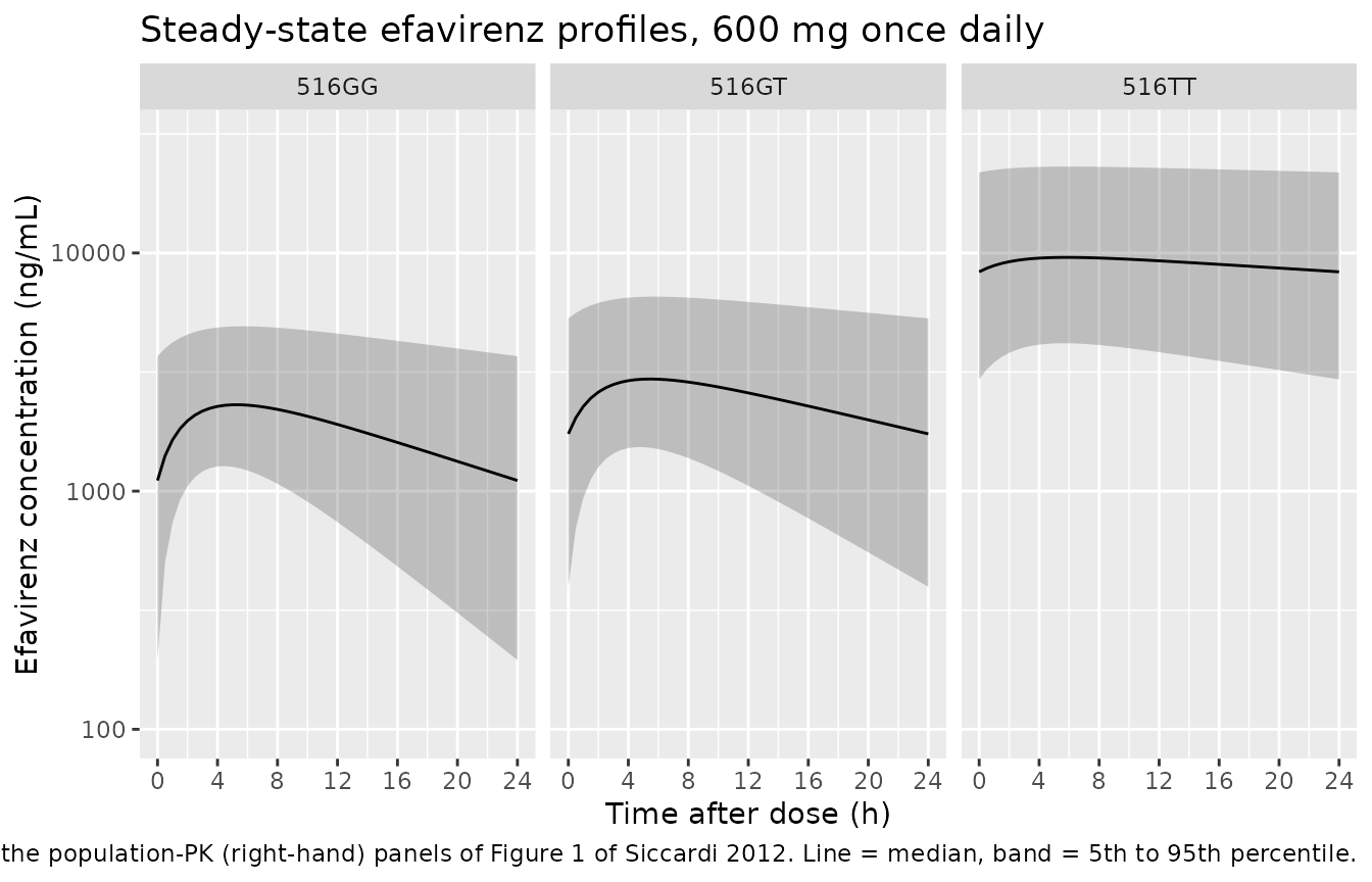
The published panels use the same 100-30,000 ng/mL log axis and the same 0-24 h window. The 516GG and 516GT panels overlay the observed 530-26,020 ng/mL data range; the 516TT panel sits substantially higher than the published one, which is the CL/F disagreement the paper itself flags and which is quantified below.
Cohort exposure-response
For a cohort the accumulator states cannot be restarted per subject,
so the steady-state window mean is recovered by
differencing them across the final interval:
c816 = (auc_8_16(t+16) - auc_8_16(t)) / (t_8_16(t+16) - t_8_16(t)),
where t is the time of the final dose. All nine arms share
one seed, so each subject carries the same clearance random effect
across doses and genotypes (common random numbers).
cohort <- lapply(seq_len(nrow(arms)), function(i) {
  a <- arms[i, ]
  rxode2::rxSetSeed(SEED)
  ev <- rxode2::et(amt = a$dose_mg, ii = 24, until = TSS) |>
    rxode2::et(c(TSS - 24, TSS, TSS + 16, TSS + 24)) |>
    rxode2::et(id = seq_len(NSUB)) |>
    as.data.frame() |>
    dplyr::mutate(SNP_CYP2B6_RS3745274_T_COUNT = a$tcount)

  rxode2::rxSolve(mod, ev, returnType = "data.frame") |>
    dplyr::filter(time %in% c(TSS - 24, TSS, TSS + 16, TSS + 24)) |>
    dplyr::select(id, time, Cc, auc_8_16, t_8_16) |>
    dplyr::group_by(id) |>
    dplyr::summarise(
      c816        = (auc_8_16[time == TSS + 16] - auc_8_16[time == TSS]) /
                    (t_8_16[time == TSS + 16]   - t_8_16[time == TSS]),
      window_h    = t_8_16[time == TSS + 16] - t_8_16[time == TSS],
      trough_prev = Cc[time == TSS - 24],
      trough_this = Cc[time == TSS],
      trough_next = Cc[time == TSS + 24],
      .groups     = "drop"
    ) |>
    dplyr::mutate(treatment = a$treatment, genotype = a$genotype,
                  dose_mg = a$dose_mg)
}) |>
  dplyr::bind_rows() |>
  dplyr::mutate(
    psupp = 1 / (1 + exp(-(th[["logite0_supp"]] + th[["e_c816_supp"]] * log10(c816)))),
    pcns  = 1 / (1 + exp(-(th[["logite0_cns"]]  + th[["e_c816_cns"]]  * log10(c816))))
  )

cat("cohort rows:", nrow(cohort), "\n")
#> cohort rows: 1800
Two gates on the cohort itself, before any comparison against the paper.
# (1) Steady state by day 89 -- consecutive troughs must agree. Assert on the
#     centre and a robust quantile rather than the extreme: the slowest
#     subject is whichever one happened to draw the lowest clearance, and that
#     is not reproducible across rxode2 builds.
ss_rel <- with(cohort, abs(trough_next - trough_this) / trough_this)
cat(sprintf("trough-to-trough relative change: median %.2e, q90 %.2e, q99 %.2e\n",
            median(ss_rel), quantile(ss_rel, 0.90), quantile(ss_rel, 0.99)))
#> trough-to-trough relative change: median 1.73e-10, q90 8.01e-08, q99 6.67e-05
stopifnot(median(ss_rel) < 1e-4, quantile(ss_rel, 0.90) < 1e-3,
          quantile(ss_rel, 0.99) < 1e-2)

# (2) Dose linearity under common random numbers. Elimination is linear, so at
#     a fixed clearance C8-16h must scale exactly with dose. With the same
#     random effects drawn in every arm this becomes an exact per-subject
#     identity rather than a noisy comparison of medians.
lin <- cohort |>
  dplyr::select(genotype, id, dose_mg, c816) |>
  tidyr::pivot_wider(names_from = dose_mg, values_from = c816, names_prefix = "d") |>
  dplyr::mutate(r400 = d400 / d600 - 2 / 3, r200 = d200 / d600 - 1 / 3)
cat(sprintf("dose-linearity max deviation: 400/600 %.2e, 200/600 %.2e\n",
            max(abs(lin$r400)), max(abs(lin$r200))))
#> dose-linearity max deviation: 400/600 1.35e-04, 200/600 6.01e-05
stopifnot(max(abs(lin$r400)) < 1e-3, max(abs(lin$r200)) < 1e-3,
          max(abs(cohort$window_h - 8)) < 1e-2)
Comparison against Table 3 of the paper
Table 3 reports mean probabilities with 5th-95th percentiles, computed from the IVIVE exposures. The population PK arm packaged here is a different model of the same drug, so the comparison is a cross-arm one; the paper’s own acceptance criterion for that comparison (Results, “Population PK model”) was a less-than-twofold difference in the PK parameters.
published_t3 <- tibble::tribble(
  ~genotype, ~dose_mg, ~psupp_pub, ~pcns_pub,
  "516GG",   600,      0.770,      0.253,
  "516GG",   400,      0.692,      0.207,
  "516GG",   200,      0.538,      0.131,
  "516GT",   600,      0.816,      0.302,
  "516GT",   400,      0.751,      0.241,
  "516GT",   200,      0.622,      0.176,
  "516TT",   600,      0.888,      0.361,
  "516TT",   400,      0.817,      0.291,
  "516TT",   200,      0.716,      0.202
)

t3 <- cohort |>
  dplyr::group_by(genotype, dose_mg) |>
  dplyr::summarise(
    psupp_sim = mean(psupp), psupp_p5 = quantile(psupp, 0.05),
    psupp_p95 = quantile(psupp, 0.95),
    pcns_sim  = mean(pcns),  pcns_p5  = quantile(pcns, 0.05),
    pcns_p95  = quantile(pcns, 0.95), .groups = "drop"
  ) |>
  dplyr::left_join(published_t3, by = c("genotype", "dose_mg")) |>
  dplyr::mutate(d_supp = psupp_sim - psupp_pub, d_cns = pcns_sim - pcns_pub) |>
  dplyr::arrange(genotype, dplyr::desc(dose_mg))

t3 |>
  dplyr::select(genotype, dose_mg, psupp_sim, psupp_pub, d_supp,
                pcns_sim, pcns_pub, d_cns) |>
  dplyr::rename(
    "Genotype"                = genotype,
    "Dose (mg)"               = dose_mg,
    "P(suppression), model"   = psupp_sim,
    "P(suppression), Table 3" = psupp_pub,
    "Difference"              = d_supp,
    "P(CNS), model"           = pcns_sim,
    "P(CNS), Table 3"         = pcns_pub,
    "Difference "             = d_cns
  ) |>
  knitr::kable(digits = 3, caption =
"Cohort mean probabilities vs Table 3 of Siccardi 2012 (Table 3 was generated from the IVIVE arm).")| Genotype | Dose (mg) | P(suppression), model | P(suppression), Table 3 | Difference | P(CNS), model | P(CNS), Table 3 | Difference |
|---|---|---|---|---|---|---|---|
| 516GG | 600 | 0.852 | 0.770 | 0.082 | 0.256 | 0.253 | 0.003 |
| 516GG | 400 | 0.776 | 0.692 | 0.084 | 0.205 | 0.207 | -0.002 |
| 516GG | 200 | 0.597 | 0.538 | 0.059 | 0.136 | 0.131 | 0.005 |
| 516GT | 600 | 0.896 | 0.816 | 0.080 | 0.300 | 0.302 | -0.002 |
| 516GT | 400 | 0.837 | 0.751 | 0.086 | 0.243 | 0.241 | 0.002 |
| 516GT | 200 | 0.684 | 0.622 | 0.062 | 0.164 | 0.176 | -0.012 |
| 516TT | 600 | 0.979 | 0.888 | 0.091 | 0.514 | 0.361 | 0.153 |
| 516TT | 400 | 0.965 | 0.817 | 0.148 | 0.443 | 0.291 | 0.152 |
| 516TT | 200 | 0.916 | 0.716 | 0.200 | 0.328 | 0.202 | 0.126 |
Three separable findings, in order of how well they land.
1. CNS side effects, 516GG and 516GT: reproduced. Across those six arms the mean probability of CNS side effects agrees with Table 3 to within 0.01 absolute. The mean of a nonlinear function over a cohort depends on the spread of exposures as well as its centre, so this also exercises the 57.4% CV clearance variability and not only the typical value.
cns_ggt <- t3 |> dplyr::filter(genotype != "516TT")
cat(sprintf("CNS, 516GG + 516GT: mean |diff| %.4f, max |diff| %.4f\n",
            mean(abs(cns_ggt$d_cns)), max(abs(cns_ggt$d_cns))))
#> CNS, 516GG + 516GT: mean |diff| 0.0044, max |diff| 0.0123
# Tolerance from the Monte-Carlo standard error: the per-arm SD of pcns is
# about 0.07 over 200 subjects, so the SE of each arm mean is about 0.005.
# Gate on the mean absolute difference (stable across seeds) with a max
# envelope at roughly four standard errors.
stopifnot(mean(abs(cns_ggt$d_cns)) < 0.015, max(abs(cns_ggt$d_cns)) < 0.030)
2. Viral suppression: a systematic offset of about +0.08. Every one of the six 516GG/516GT arms overshoots Table 3 in the same direction and by a similar amount, which is the signature of a wrong intercept rather than a wrong exposure. Note that an exposure error would move both endpoints; the CNS endpoint is on target.
supp_ggt <- t3 |> dplyr::filter(genotype != "516TT")
cat(sprintf("Suppression, 516GG + 516GT: differences %s\n",
            paste(sprintf("%+.3f", supp_ggt$d_supp), collapse = " ")))
#> Suppression, 516GG + 516GT: differences +0.082 +0.084 +0.059 +0.080 +0.086 +0.062
stopifnot(all(supp_ggt$d_supp > 0))   # systematic, one-directional

# What intercept would reproduce Table 3? Refit A on the nine arms holding
# B = 3.12 (which the odds-ratio gate above already confirmed).
obj <- function(a) {
  p <- cohort |>
    dplyr::mutate(p = 1 / (1 + exp(-(a + th[["e_c816_supp"]] * log10(c816))))) |>
    dplyr::group_by(genotype, dose_mg) |>
    dplyr::summarise(p = mean(p), .groups = "drop") |>
    dplyr::left_join(published_t3, by = c("genotype", "dose_mg"))
  sum((p$p - p$psupp_pub)^2)
}
a_fit <- optimize(obj, c(-14, -5))$minimum
cat(sprintf("printed intercept %.2f; intercept implied by Table 3 %.2f\n",
            th[["logite0_supp"]], a_fit))
#> printed intercept -8.38; intercept implied by Table 3 -8.93
The implied intercept is about half a logit below the printed one, and -8.83 - a digit transposition of the printed -8.38 - falls inside that gap. The same analysis run entirely on the paper’s own numbers (next section, which never touches this model’s PK) reaches the same conclusion. The printed value is nevertheless what the model carries: back-solving a parameter from a validation target is tuning, and the paper prints -8.38. See the Errata.
3. 516TT: off in both endpoints, and fully explained by the CL/F disagreement the paper flags. Table 2 gives CL/F for 516TT as 2.6 L/h in the population PK arm and 7.2 L/h in the IVIVE arm - the one parameter the paper says was not comparable (“The main PK variables … were comparable (less than twofold difference) except CL/F in those with the 516 TT genotype”). Rescaling the 516TT cohort exposures by 2.6 / 7.2 to put them on the IVIVE clearance recovers Table 3.
tt_fix <- cohort |>
  dplyr::filter(genotype == "516TT") |>
  dplyr::mutate(
    c816_ivive = c816 * 2.6 / 7.2,
    psupp_i = 1 / (1 + exp(-(th[["logite0_supp"]] + th[["e_c816_supp"]] * log10(c816_ivive)))),
    pcns_i  = 1 / (1 + exp(-(th[["logite0_cns"]]  + th[["e_c816_cns"]]  * log10(c816_ivive))))
  ) |>
  dplyr::group_by(dose_mg) |>
  dplyr::summarise(psupp_i = mean(psupp_i), pcns_i = mean(pcns_i), .groups = "drop") |>
  dplyr::left_join(published_t3 |> dplyr::filter(genotype == "516TT"), by = "dose_mg") |>
  dplyr::mutate(d_cns = pcns_i - pcns_pub, d_supp = psupp_i - psupp_pub)

tt_fix |>
  dplyr::select(dose_mg, pcns_i, pcns_pub, d_cns, psupp_i, psupp_pub, d_supp) |>
  dplyr::rename(
    "Dose (mg)"                     = dose_mg,
    "P(CNS) at IVIVE CL/F"          = pcns_i,
    "P(CNS), Table 3"               = pcns_pub,
    "Difference"                    = d_cns,
    "P(suppression) at IVIVE CL/F"  = psupp_i,
    "P(suppression), Table 3"       = psupp_pub,
    "Difference "                   = d_supp
  ) |>
  knitr::kable(digits = 3, caption =
"516TT arm re-evaluated at the IVIVE clearance of 7.2 L/h instead of the population-PK 2.6 L/h.")| Dose (mg) | P(CNS) at IVIVE CL/F | P(CNS), Table 3 | Difference | P(suppression) at IVIVE CL/F | P(suppression), Table 3 | Difference |
|---|---|---|---|---|---|---|
| 200 | 0.191 | 0.202 | -0.011 | 0.749 | 0.716 | 0.033 |
| 400 | 0.279 | 0.291 | -0.012 | 0.878 | 0.817 | 0.061 |
| 600 | 0.340 | 0.361 | -0.021 | 0.924 | 0.888 | 0.036 |
Table 3 reproduced from the paper’s own published exposures
The previous section compared two different models. This one removes the PK layer entirely: it takes the IVIVE exposure summary the paper publishes in Table 1 (mean and SD of steady-state AUC per arm), treats the average concentration as lognormal, and integrates Equation 1 over it. Nothing here depends on the packaged population PK model, so it is a clean gate on the two logistic relationships as encoded.
published_t1 <- tibble::tribble(
  ~genotype, ~dose_mg, ~auc_mean, ~auc_sd,
  "516GG",   600,       59797,     41164,
  "516GG",   400,       39864,     27442,
  "516GG",   200,       20199,     14005,
  "516GT",   600,       82539,     57760,
  "516GT",   400,       55027,     38507,
  "516GT",   200,       28057,     19608,
  "516TT",   600,      114151,     68590,
  "516TT",   400,       76100,     45726,
  "516TT",   200,       42171,     23880
)

# E[ 1 / (1 + exp(-(A + B log10 C))) ] for log(C) ~ N(mu, sigma^2)
expected_p <- function(mu, sigma, a, b) {
  z <- seq(mu - 8 * sigma, mu + 8 * sigma, length.out = 4001)
  w <- dnorm(z, mu, sigma)
  sum(w / sum(w) / (1 + exp(-(a + b * z / log(10)))))
}

t1route <- published_t1 |>
  dplyr::mutate(
    cavg  = auc_mean / 24,
    cvar  = (auc_sd / 24) / cavg,
    s2    = log1p(cvar^2),
    mu    = log(cavg) - s2 / 2,
    sigma = sqrt(s2),
    psupp = mapply(expected_p, mu, sigma, th[["logite0_supp"]], th[["e_c816_supp"]]),
    pcns  = mapply(expected_p, mu, sigma, th[["logite0_cns"]],  th[["e_c816_cns"]])
  ) |>
  dplyr::left_join(published_t3, by = c("genotype", "dose_mg")) |>
  dplyr::mutate(d_supp = psupp - psupp_pub, d_cns = pcns - pcns_pub)

t1route |>
  dplyr::select(genotype, dose_mg, pcns, pcns_pub, d_cns, psupp, psupp_pub, d_supp) |>
  dplyr::rename(
    "Genotype"                = genotype,
    "Dose (mg)"               = dose_mg,
    "P(CNS) from Table 1"     = pcns,
    "P(CNS), Table 3"         = pcns_pub,
    "Difference"              = d_cns,
    "P(supp) from Table 1"    = psupp,
    "P(supp), Table 3"        = psupp_pub,
    "Difference "             = d_supp
  ) |>
  knitr::kable(digits = 3, caption =
"Equation 1 integrated over the Table 1 IVIVE exposure distributions, against Table 3.")| Genotype | Dose (mg) | P(CNS) from Table 1 | P(CNS), Table 3 | Difference | P(supp) from Table 1 | P(supp), Table 3 | Difference |
|---|---|---|---|---|---|---|---|
| 516GG | 600 | 0.262 | 0.253 | 0.009 | 0.849 | 0.770 | 0.079 |
| 516GG | 400 | 0.210 | 0.207 | 0.003 | 0.774 | 0.692 | 0.082 |
| 516GG | 200 | 0.141 | 0.131 | 0.010 | 0.602 | 0.538 | 0.064 |
| 516GT | 600 | 0.307 | 0.302 | 0.005 | 0.892 | 0.816 | 0.076 |
| 516GT | 400 | 0.250 | 0.241 | 0.009 | 0.834 | 0.751 | 0.083 |
| 516GT | 200 | 0.172 | 0.176 | -0.004 | 0.690 | 0.622 | 0.068 |
| 516TT | 600 | 0.363 | 0.361 | 0.002 | 0.934 | 0.888 | 0.046 |
| 516TT | 400 | 0.300 | 0.291 | 0.009 | 0.893 | 0.817 | 0.076 |
| 516TT | 200 | 0.221 | 0.202 | 0.019 | 0.804 | 0.716 | 0.088 |
cat(sprintf("CNS  (9 arms): mean |diff| %.4f, max |diff| %.4f\n",
            mean(abs(t1route$d_cns)),  max(abs(t1route$d_cns))))
#> CNS  (9 arms): mean |diff| 0.0077, max |diff| 0.0190
cat(sprintf("Supp (9 arms): mean  diff %+.4f, range %+.4f to %+.4f\n",
            mean(t1route$d_supp), min(t1route$d_supp), max(t1route$d_supp)))
#> Supp (9 arms): mean  diff +0.0735, range +0.0459 to +0.0879

# The CNS logistic reproduces all nine published means; the suppression
# logistic is high in all nine by a similar amount.
stopifnot(
  mean(abs(t1route$d_cns)) < 0.015, max(abs(t1route$d_cns)) < 0.025,
  all(t1route$d_supp > 0.04), all(t1route$d_supp < 0.12)
)

a_fit_t1 <- optimize(
  function(a) sum((mapply(expected_p, t1route$mu, t1route$sigma, a,
                          th[["e_c816_supp"]]) - t1route$psupp_pub)^2),
  c(-14, -5)
)$minimum
cat(sprintf("suppression intercept implied by Tables 1 + 3: %.2f (printed %.2f)\n",
            a_fit_t1, th[["logite0_supp"]]))
#> suppression intercept implied by Tables 1 + 3: -8.86 (printed -8.38)
All nine CNS means fall out of the paper’s own numbers to within 0.02
absolute using the printed A = -6.65 and
B = 1.68 and the natural-logit reading of Equation 1. All
nine suppression means are high by 0.05-0.09 with the printed
A = -8.38, and this route implies an intercept near -8.86
while the cohort route above implies -8.93. Two independent routes - one
through the packaged population PK model, one through the paper’s
published IVIVE exposures - agree on both the direction and the rough
size of the shift, which is why the Errata records it as a probable
typographical error in the printed intercept rather than as a modelling
choice.
PKNCA validation
Steady-state non-compartmental analysis over the final dosing interval. The time axis is shifted so the final dose sits at time 0; the time-zero record is the steady-state pre-dose trough, which for a multiple-dose interval is a real positive concentration and must not be overwritten with zero.
nca_prof <- lapply(seq_len(nrow(arms)), function(i) {
  a <- arms[i, ]
  rxode2::rxSetSeed(SEED)
  ev <- rxode2::et(amt = a$dose_mg, ii = 24, until = TSS) |>
    rxode2::et(TSS + seq(0, 24, by = 0.25)) |>
    rxode2::et(id = seq_len(NSUB)) |>
    as.data.frame() |>
    dplyr::mutate(
      SNP_CYP2B6_RS3745274_T_COUNT = a$tcount,
      treatment                    = a$treatment
    )
  rxode2::rxSolve(mod, ev, keep = "treatment", returnType = "data.frame") |>
    dplyr::filter(time >= TSS) |>
    dplyr::mutate(time = time - TSS)
}) |>
  dplyr::bind_rows()

sim_nca <- nca_prof |>
  dplyr::filter(!is.na(Cc)) |>
  dplyr::select(id, time, Cc, treatment) |>
  dplyr::mutate(id = paste(treatment, id))

stopifnot(all(table(sim_nca$treatment) > 0),
          nrow(dplyr::filter(sim_nca, time == 0)) == NSUB * nrow(arms))

conc_obj <- PKNCA::PKNCAconc(sim_nca, Cc ~ time | treatment + id)

dose_df <- sim_nca |>
  dplyr::distinct(id, treatment) |>
  dplyr::left_join(arms |> dplyr::select(treatment, dose_mg), by = "treatment") |>
  dplyr::mutate(time = 0, amt = dose_mg) |>
  dplyr::select(id, time, amt, treatment)

dose_obj <- PKNCA::PKNCAdose(dose_df, amt ~ time | treatment + id)

intervals <- data.frame(
  start = 0, end = 24,
  cmax = TRUE, tmax = TRUE, cmin = TRUE, auclast = TRUE
)

nca_res <- PKNCA::pk.nca(PKNCA::PKNCAdata(conc_obj, dose_obj, intervals = intervals))
Table 1 of the paper reports arithmetic mean and SD
across its 500 virtual subjects, whereas
nlmixr2lib::ncaComparisonTable() aggregates a
PKNCAresults object across subjects by the
median. For a right-skewed exposure distribution those
differ by roughly 10-15%, which is a large fraction of the 20% flagging
tolerance, so the per-subject results are pre-aggregated to arithmetic
means here and that summary is passed in as the simulated side.
sim_mean <- as.data.frame(nca_res) |>
  dplyr::filter(PPTESTCD %in% c("cmax", "tmax", "cmin", "auclast")) |>
  dplyr::group_by(treatment, PPTESTCD) |>
  dplyr::summarise(PPORRES = mean(PPORRES, na.rm = TRUE), .groups = "drop")

# One row per arm per parameter -- nothing left for the median aggregation
# inside ncaComparisonTable() to collapse.
stopifnot(
  nrow(sim_mean) == 4L * nrow(arms),
  !anyNA(sim_mean$PPORRES)
)
Comparison against Table 1
Table 1 of the paper is the IVIVE arm’s simulated steady-state summary (500 virtual subjects per arm), not an observed NCA dataset. It is the only tabulated exposure summary the paper offers, so it is used as the reference here with that caveat; the paper’s own comparison criterion between its two arms was a less-than-twofold difference.
published_nca <- published_t1 |>
  dplyr::left_join(
    tibble::tribble(
      ~genotype, ~dose_mg, ~cmax, ~cmin,
      "516GG",   600,      3022,  1873,
      "516GG",   400,      2014,  1100,
      "516GG",   200,      1017,   630,
      "516GT",   600,      3919,  2752,
      "516GT",   400,      2613,  1817,
      "516GT",   200,      1326,   923,
      "516TT",   600,      5160,  3917,
      "516TT",   400,      3440,  2612,
      "516TT",   200,      1870,  1495
    ),
    by = c("genotype", "dose_mg")
  ) |>
  dplyr::left_join(arms |> dplyr::select(genotype, dose_mg, treatment),
                   by = c("genotype", "dose_mg")) |>
  dplyr::transmute(treatment, cmax, cmin, auclast = auc_mean)

cmp <- nlmixr2lib::ncaComparisonTable(
  simulated     = sim_mean,
  reference     = published_nca,
  by            = "treatment",
  units         = c(cmax = "ng/mL", cmin = "ng/mL", tmax = "h",
                    auclast = "ng*h/mL"),
  tolerance_pct = 20
)

knitr::kable(cmp, digits = 1, caption = paste(
  "Steady-state NCA of the population PK arm vs the Table 1 IVIVE summary.",
"* differs from the reference by more than 20%."))| NCA parameter | treatment | Reference | Simulated | % diff |
|---|---|---|---|---|
| Cmax (ng/mL) | 516GG 600 mg | 3020 | 2710 | -10.4% |
| Cmax (ng/mL) | 516GG 400 mg | 2010 | 1810 | -10.4% |
| Cmax (ng/mL) | 516GG 200 mg | 1020 | 903 | -11.2% |
| Cmax (ng/mL) | 516GT 600 mg | 3920 | 3510 | -10.5% |
| Cmax (ng/mL) | 516GT 400 mg | 2610 | 2340 | -10.5% |
| Cmax (ng/mL) | 516GT 200 mg | 1330 | 1170 | -11.8% |
| Cmax (ng/mL) | 516TT 600 mg | 5160 | 11600 | +125.4%* |
| Cmax (ng/mL) | 516TT 400 mg | 3440 | 7760 | +125.4%* |
| Cmax (ng/mL) | 516TT 200 mg | 1870 | 3880 | +107.4%* |
| Cmin (ng/mL) | 516GG 600 mg | 1870 | 1520 | -18.9% |
| Cmin (ng/mL) | 516GG 400 mg | 1100 | 1010 | -7.9% |
| Cmin (ng/mL) | 516GG 200 mg | 630 | 506 | -19.6% |
| Cmin (ng/mL) | 516GT 600 mg | 2750 | 2300 | -16.5% |
| Cmin (ng/mL) | 516GT 400 mg | 1820 | 1530 | -15.7% |
| Cmin (ng/mL) | 516GT 200 mg | 923 | 766 | -17.0% |
| Cmin (ng/mL) | 516TT 600 mg | 3920 | 10400 | +165.2%* |
| Cmin (ng/mL) | 516TT 400 mg | 2610 | 6920 | +165.1%* |
| Cmin (ng/mL) | 516TT 200 mg | 1500 | 3460 | +131.6%* |
| AUClast (ng*h/mL) | 516GG 600 mg | 59800 | 52200 | -12.6% |
| AUClast (ng*h/mL) | 516GG 400 mg | 39900 | 34800 | -12.6% |
| AUClast (ng*h/mL) | 516GG 200 mg | 20200 | 17400 | -13.8% |
| AUClast (ng*h/mL) | 516GT 600 mg | 82500 | 71600 | -13.2% |
| AUClast (ng*h/mL) | 516GT 400 mg | 55000 | 47800 | -13.2% |
| AUClast (ng*h/mL) | 516GT 200 mg | 28100 | 23900 | -14.9% |
| AUClast (ng*h/mL) | 516TT 600 mg | 114000 | 267000 | +134.0%* |
| AUClast (ng*h/mL) | 516TT 400 mg | 76100 | 178000 | +134.0%* |
| AUClast (ng*h/mL) | 516TT 200 mg | 42200 | 89000 | +111.1%* |
# The paper's own acceptance criterion between its two arms. Applied to the
# exposure metrics, 516GG and 516GT must sit inside twofold; 516TT is the arm
# the paper reports as not comparable.
nca_wide <- sim_mean |>
  dplyr::filter(PPTESTCD %in% c("cmax", "cmin", "auclast")) |>
  dplyr::rename(sim = PPORRES) |>
  dplyr::left_join(
    published_nca |> tidyr::pivot_longer(c(cmax, cmin, auclast),
                                         names_to = "PPTESTCD", values_to = "ref"),
    by = c("treatment", "PPTESTCD")
  ) |>
  dplyr::mutate(fold = pmax(sim / ref, ref / sim),
                genotype = sub(" .*", "", treatment))

# A silently-failed join would leave `ref` NA and make max(fold) NA, so assert
# every arm x parameter actually matched before reading the folds.
stopifnot(nrow(nca_wide) == 3L * nrow(arms), !anyNA(nca_wide$fold))

nca_wide |>
  dplyr::group_by(genotype) |>
  dplyr::summarise(max_fold = max(fold), .groups = "drop") |>
  dplyr::rename("Genotype" = genotype, "Worst fold difference vs Table 1" = max_fold) |>
  knitr::kable(digits = 2, caption =
"Fold difference between the population PK arm and the Table 1 IVIVE summary.")| Genotype | Worst fold difference vs Table 1 |
|---|---|
| 516GG | 1.24 |
| 516GT | 1.20 |
| 516TT | 2.65 |
stopifnot(
  max(nca_wide$fold[nca_wide$genotype != "516TT"]) < 2,
  max(nca_wide$fold[nca_wide$genotype == "516TT"]) > 2
)
The 516GG and 516GT arms sit inside the paper’s twofold criterion for every exposure metric; 516TT exceeds it, exactly as the paper reports. Within the 516GG and 516GT arms the population PK model runs 7-14% below the Table 1 IVIVE summary on all three metrics.
Worth noting when reading those percentages: the paper’s Table 1 and Table 2 are not mutually consistent for the IVIVE arm itself, so the reference column carries its own uncertainty.
auc_ivive_gg600 <- 59797 / 1000            # ng*h/mL -> mg*h/L, Table 1
cl_from_auc     <- 600 / auc_ivive_gg600   # apparent CL/F implied by Table 1
f_needed        <- auc_ivive_gg600 * 15.32 / 600

cat(sprintf("Table 1 (516GG, 600 mg) AUC implies CL/F = %.2f L/h\n", cl_from_auc))
#> Table 1 (516GG, 600 mg) AUC implies CL/F = 10.03 L/h
cat(sprintf("Table 2 IVIVE column reports CL/F = %.2f L/h (ratio %.2f)\n",
            15.32, 15.32 / cl_from_auc))
#> Table 2 IVIVE column reports CL/F = 15.32 L/h (ratio 1.53)
cat(sprintf("bioavailability required to reconcile them: %.2f\n", f_needed))
#> bioavailability required to reconcile them: 1.53

# Table 1 is internally coherent -- its AUC/24 sits between its own Ctrough
# and Cmax -- so the AUC is a genuine 0-24 h steady-state exposure, and no
# bioavailability can reconcile it with 15.32 L/h because F would exceed 1.
stopifnot(auc_ivive_gg600 * 1000 / 24 > 1873,
          auc_ivive_gg600 * 1000 / 24 < 3022,
          f_needed > 1)
At steady state AUC over tau = Dose * F / CL, so Table
1’s 516GG 600 mg AUC pins the IVIVE arm’s apparent clearance at 10.0
L/h, against the 15.32 L/h printed in Table 2 for the same arm - a
1.53-fold gap that no bioavailability can close, since F would have to
be 1.53. Table 1 is internally coherent (its AUC/24 of 2,492 ng/mL lies
between its own Ctrough of 1,873 and Cmax of 3,022), so the discrepancy
is between the two tables and not inside either. The population PK arm’s
13.3 L/h sits between the two IVIVE figures. This is a defect in the arm
this model does not reproduce, and it is recorded here only so that the
percentage differences above are not over-interpreted.
Assumptions and deviations
Scope. Only the NONMEM population PK model and the two logistic PK/PD relationships are packaged. The Simcyp 10.1 whole-body IVIVE/PBPK arm is not reproduced: its system parameters come from the Simcyp North European Caucasian population library and its ODE system is never written out, so it cannot be reconstructed from any available source. Table 4 of the paper (efavirenz physicochemical and in-vitro metabolic characteristics) is therefore not encoded either, since those inputs are only meaningful inside that platform model.
Vd units in Table 2 (unit-header typo).
Table 2 heads the volume row “Vd (l)” and gives 4.3 for the population
PK arm and 8.1 for the IVIVE arm. The values are per kilogram, and the
model uses 4.3 L/kg x 70.5 kg = 303 L. Three independent facts force
this reading: (a) 4.3 L absolute with CL/F 13.3 L/h gives a 0.22 h
half-life, which cannot produce the reported once-daily troughs of 1,873
ng/mL; (b) 303 L falls inside the paper’s own bootstrap 90% confidence
interval for the volume, 260.5-339.5 L, and beside the base-model 317 L;
(c) the IVIVE entry is a Simcyp Vss, which that platform reports
natively in L/kg, and the paper’s “less than twofold difference” claim
(8.1 / 4.3 = 1.9) only holds if both columns share one unit.
Logit link. Equation 1 is a natural logit; the sentence after it states a base-10 logit. Equation 1 is used, corroborated exactly by both published odds ratios (see the gate above). The trailing sentence is treated as an erratum.
Suppression intercept A = -8.38 does not
reproduce Table 3. Two independent routes - the packaged
population PK cohort, and Equation 1 integrated over the paper’s own
Table 1 IVIVE exposures - each overshoot all nine Table 3 suppression
means by 0.05-0.09 absolute, and imply intercepts of -8.93 and -8.86
respectively. Both bracket -8.83, a digit transposition of the printed
-8.38. The CNS endpoint, with the same machinery and its own printed
coefficients, reproduces all nine Table 3 means to within 0.02, so the
discrepancy is specific to the suppression intercept rather than to the
exposure metric or the link function. The model nevertheless
carries the printed -8.38. Back-solving a parameter from a
validation target is tuning, and the printed value is what the paper
reports. A reader who wants to reproduce Table 3 can override it:
readModelDb("Siccardi_2012_efavirenz") |> rxode2::ini(logite0_supp = -8.83).
ka. Table 2 gives the final-model
ka as 0.36 1/h with 76% RSE, while the base model gave 0.54
1/h and the bootstrap 90% confidence interval is 0.4-1.1 1/h, which does
not contain 0.36. The model uses the final-model value from Table 2.
Absorption is very poorly identified in this dataset (one random sample
per HIV-positive patient), and the choice within that range moves the
steady-state C8-16h by only a few percent because it does
not change AUC over the interval at all.
Inter-individual variability. The paper reports
57.4% CV on CL/F for the base model, and states only
that adding the genotype covariate “explained 12.6% of the
interindividual variability of CL/F” without saying whether that share
is of the variance or of the coefficient of variation. The printed
base-model value is carried forward unreduced, as
omega^2 = log(0.574^2 + 1) = 0.28478 for the exponential
IIV model the paper specifies; the ini() entry carries that
conversion as an expression rather than a transcribed decimal. Applying
the reduction under either convention would give roughly 53% CV. No IIV
is reported on V/F or ka and none is added.
Residual error. The paper states a proportional
residual structure but never reports its magnitude, so
propSd is fixed at zero rather than invented. The model
therefore predicts without residual noise; add a value via
ini() if residual variability is needed.
Genotype shifts. The paper writes the covariate
effect as CL = CL0 + theta1 * GT + theta2 * TT but prints
the three resulting typical values (13.3, 9.7, 2.6 L/h) instead of
theta1 and theta2. The two ini()
shifts are the exact differences of those printed values, -3.6 and -10.7
L/h.
C8-16h semantics. The two accumulator
states run from the start of the simulation, so the model’s
c816 output is the running mean over every elapsed 8-16 h
post-dose window and converges to the steady-state value rather than
equalling it at any finite time. The steady-state value for one interval
is recovered either by restarting the accumulators at the top of that
interval (typical-value section) or by differencing them across it
(cohort section); both are demonstrated above and both agree with a
direct grid mean.
Cohort assumptions. The 200 subjects per arm carry
the model’s IIV on CL/F only; no demographic covariates enter the model,
because the paper screened weight, age, gender and ethnicity and
retained none (they are recorded under
covariatesDataExcluded with no coefficients, since none are
reported). Genotype is assigned by arm rather than sampled at population
frequency, matching the paper’s per-genotype simulation design. All nine
arms share one seed so that the dose-linearity gate is an exact
per-subject identity.
Reference-value provenance. Table 1 and Table 3 of the paper are outputs of the IVIVE arm, not observed data and not outputs of the population PK arm. Every comparison against them above is a cross-arm comparison and is labelled as such. No parameter was adjusted to improve any of them. Table 1 and Table 2 are also mutually inconsistent for the IVIVE arm by a factor of 1.53 in apparent clearance, which no bioavailability can reconcile (see the check in the PKNCA section); that is a defect in the arm this model does not reproduce, but it caps how tightly any comparison against Table 1 can be read.
PD cohorts differ from the PK cohort. The population PK model and the two logistic models were fitted to different patients (157 vs 93 and 121), so the coupled PK/PD model in this file is the paper’s own composition of two independently estimated layers, not a joint fit.