Perioperative factor VIII (Preijers 2021)
Source:vignettes/articles/Preijers_2021_factor_viii.Rmd
Preijers_2021_factor_viii.RmdModel and source
- Citation: Preijers T, Liesner R, Hazendonk HCAM, Chowdary P, Driessens MHE, Hart DP, Laros-van Gorkom BAP, van der Meer FJM, Meijer K, Fijnvandraat K, Leebeek FWG, Mathot RAA, Cnossen MH; OPTI-CLOT study group. Validation of a perioperative population factor VIII pharmacokinetic model with a large cohort of pediatric hemophilia A patients. Br J Clin Pharmacol. 2021;87(11):4408-4420. doi:[10.1111/bcp.14864](https://doi.org/10.1111/bcp.14864). PMID:33884664.
- Description: two-compartment population PK model for perioperative
factor VIII (FVIII) concentrates in children and adults with hemophilia
A. The paper first externally validated the Hazendonk 2016 perioperative
model (
Hazendonk_2016_factor_viiiin this package) on 87 children from Great Ormond Street Hospital (GOSH), found that it under-predicted their FVIII levels, and then re-estimated the model on the pooled original and new data. The re-estimated final model is packaged here. - Modality: recombinant (88% of procedures) and plasma-derived FVIII concentrates given by intravenous bolus or continuous infusion; FVIII activity measured by one-stage clotting assay in IU/mL.
The final model (Preijers 2021 Table 2 footnote) is
with BG = 1 for blood group O. The measured FVIII level
is the model prediction plus the patient’s endogenous baseline level,
reduced by 30% for samples from patients on the B-domain-deleted product
Refacto AF (Methods Eq. 1; see Assumptions and deviations for how that
equation is read).
Population
The final model was fitted to 206 patients undergoing 342 surgical procedures (Preijers 2021 Table 1):
- the original cohort of Hazendonk 2016: 119 patients (children and adults) from five Dutch hemophilia treatment centres, median age 39.6 years (0.24-77.6), median weight 75 kg (5-111), 70% severe hemophilia A, 197 procedures of which 49% were major surgery and 59% used continuous infusion;
- the new cohort: 87 children from GOSH, London, median age 2.57 years (0.03-15.2), median weight 14 kg (4-57), all with severe hemophilia A, 145 minor procedures to insert, replace or remove a central venous access device, all dosed by bolus.
The total cohort had a median age of 7.79 years (0.03-77.6) and median weight of 30 kg (4-111); 83% had severe hemophilia A and 39% blood group O (of 175 with a recorded blood group). Recombinant FVIII was used in 88% of procedures. There were 2092 FVIII measurements (one-stage clotting assay), none below the 0.01 IU/mL quantification limit.
The same information is available programmatically via
readModelDb("Preijers_2021_factor_viii")()$population.
Source trace
| Model element | Value | Source location |
|---|---|---|
lcl (CL at 68 kg, 40 y, non-O) |
log(0.171 L/h) | Table 2 final model: 171 mL/h/68 kg (RSE 7%) |
lvc (V1 at 68 kg, 40 y) |
log(2.930 L) | Table 2 final model: 2930 mL/68 kg (RSE 4%) |
lq (Q2 at 68 kg) |
log(0.172 L/h) | Table 2 final model: 172 mL/h/68 kg (RSE 19%) |
lvp (V2 at 68 kg) |
log(1.810 L) | Table 2 final model: 1810 mL/68 kg (RSE 10%) |
theta_bdp (Refacto AF fraction) |
0.30 | Table 2 final model: ‘B-domain deleted recombinant factor VIII’ 0.30 (RSE 14%) |
e_age_cl |
-0.12 | Table 2 final model ‘CL - Age’ (RSE 26%); footnote
(AGE/40)^-0.12
|
e_age_vc |
-0.09 | Table 2 final model ‘V1 - Age’ (RSE 24%); footnote
(AGE/40)^-0.09
|
e_blood_cl |
0.14 | Table 2 final model ‘CL - Blood group O’ 14% (RSE 6%); footnote
1.14^BG
|
e_wt_cl, e_wt_vc (fixed) |
0.75, 1.0 | Methods after Eq. 2: exponents fixed to 0.75 (CL, Q2) and 1 (V1, V2) |
etalcl, etalvc block |
0.14568, 0.05833, 0.07290 | Table 2 final model: IIV CL 39.6 %CV, IIV V1 27.5 %CV, correlation 56.6%; omega^2 = log(1 + CV^2), cov = r sqrt(omega^2_CL omega^2_V1) |
addSd_center123 / _center45 /
_center6
|
0.12 / 0.06 / 0.17 IU/mL | Table 2 final model: additive SD by centre |
propSd_center123 / _center45 /
_center6
|
0.197 / 0.21 / 0.22 | Table 2 final model: proportional %CV by centre |
| Two-compartment structure, 68 kg normalisation | – | Results 3.3; Methods Eq. 2 |
| Age power model | – | Methods Eq. 5; Results 3.3 (power form performed best) |
| Blood group O on CL | – | Methods Eq. 3; Table 2 footnote |
| Baseline + Refacto AF observation equation | Cc = (central/vc/1000 + FVIIIRECENT) * (1 - 0.30 * FORM_FVIII_BDD) |
Methods Eq. 1 |
Covariates tested but not retained: major surgery on CL (significant in the multivariate step, dropped after the bootstrap because its confidence interval contained 1; Results 3.4) and severe hemophilia (dropped in the multivariate analysis; Results 3.3). Inter-occasion variability on CL and V1 was tested and omitted because the model became unstable (Results 3.3).
Typical-value checks against the paper’s numbers
The Table 2 footnote equations can be evaluated directly. The Results also quote typical values for a one-year-old 10 kg non-O child under both the Hazendonk 2016 model and the present one.
mod <- readModelDb("Preijers_2021_factor_viii")
mod_hz <- readModelDb("Hazendonk_2016_factor_viii")

typ_cl <- function(wt, age, bg = 0) 171 * (wt / 68)^0.75 * (age / 40)^-0.12 * 1.14^bg
typ_v1 <- function(wt, age) 2930 * (wt / 68) * (age / 40)^-0.09
hz_cl <- function(wt, age) 150 * (wt / 68)^0.75 * (age / 40)^-0.17
hz_v1 <- function(wt, age) 2810 * (wt / 68) * (age / 40)^-0.09

# The packaged model must reproduce the footnote equations exactly.
chk_cov <- data.frame(
  id = 1:4,
  WT = c(68, 68, 10, 30),
  AGE = c(40, 40, 1, 8),
  BLOOD_GROUP_O = c(0, 1, 0, 0),
  FORM_FVIII_BDD = 0, FVIIIRECENT = 0, STUDY_OPTICLOT_CTR45 = 0, STUDY_GOSH = 0
)
ev_chk <- merge(chk_cov, data.frame(time = c(0, 1)))
ev_chk$evid <- ifelse(ev_chk$time == 0, 1L, 0L)
ev_chk$amt <- ifelse(ev_chk$evid == 1L, 1000, 0)
ev_chk$cmt <- "central"
ev_chk <- ev_chk[order(ev_chk$id, ev_chk$time), ]
sim_chk <- as.data.frame(rxSolve(zeroRe(mod), ev_chk, keep = c("WT", "AGE", "BLOOD_GROUP_O")))
#> ℹ parameter labels from comments will be replaced by 'label()'
#> Warning: No sigma parameters in the model
#> ℹ omega/sigma items treated as zero: 'etalcl', 'etalvc'
#> Warning: multi-subject simulation without without 'omega'
sim_chk <- sim_chk[!duplicated(sim_chk$id), ]
ref_cl <- typ_cl(sim_chk$WT, sim_chk$AGE, sim_chk$BLOOD_GROUP_O)
ref_v1 <- typ_v1(sim_chk$WT, sim_chk$AGE)
stopifnot(
  all(abs(sim_chk$cl * 1000 / ref_cl - 1) < 1e-8),
  all(abs(sim_chk$vc * 1000 / ref_v1 - 1) < 1e-8)
)

tibble::tibble(
  Quantity = c(
    "CL, 68 kg, 40 y, non-O (mL/h)",
    "V1, 68 kg, 40 y (mL)",
    "CL, 1 y, 10 kg, non-O: Hazendonk 2016 model (mL/h)",
    "CL, 1 y, 10 kg, non-O: Preijers 2021 model (mL/h)",
    "V1, 1 y, 10 kg: Hazendonk 2016 model (mL)",
    "V1, 1 y, 10 kg: Preijers 2021 model (mL)"
  ),
  Computed = round(c(
    typ_cl(68, 40), typ_v1(68, 40),
    hz_cl(10, 1), typ_cl(10, 1),
    hz_v1(10, 1), typ_v1(10, 1)
  ), 1),
  `Paper` = c(
    "171 (Table 2)", "2930 (Table 2)",
    "63.2 as 'from' value (Results 3.4)", "66.7 as 'to' value (Results 3.4)",
    "601 as 'from' value (Results 3.4)", "576 as 'to' value (Results 3.4)"
  )
) |>
knitr::kable(caption = "Typical values from the packaged model versus the numbers quoted in Preijers 2021.")| Quantity | Computed | Paper |
|---|---|---|
| CL, 68 kg, 40 y, non-O (mL/h) | 171.0 | 171 (Table 2) |
| V1, 68 kg, 40 y (mL) | 2930.0 | 2930 (Table 2) |
| CL, 1 y, 10 kg, non-O: Hazendonk 2016 model (mL/h) | 66.7 | 63.2 as ‘from’ value (Results 3.4) |
| CL, 1 y, 10 kg, non-O: Preijers 2021 model (mL/h) | 63.2 | 66.7 as ‘to’ value (Results 3.4) |
| V1, 1 y, 10 kg: Hazendonk 2016 model (mL) | 575.9 | 601 as ‘from’ value (Results 3.4) |
| V1, 1 y, 10 kg: Preijers 2021 model (mL) | 600.5 | 576 as ‘to’ value (Results 3.4) |
The four one-year-old values are reproduced to the printed precision, but attached to the opposite model: the Hazendonk 2016 equations give 66.7 mL/h and 576 mL and the Preijers 2021 equations give 63.2 mL/h and 601 mL, whereas Results 3.4 says CL “increased from 63.2 to 66.7” and V1 was “reduced from 601 to 576”. The numbers themselves confirm the Table 2 footnote equations; the from/to wording in the text is swapped. The Table 2 equations are used here.
Virtual cohort
Observed data are not public. Two virtual cohorts of 100 patients each mimic Table 1: a pediatric arm resembling the GOSH cohort and an adult arm resembling the adults of the original cohort. Pediatric weight follows an approximate median weight-for-age curve with 12% log-normal scatter.
set.seed(2021)
rxode2::rxSetSeed(2021)
n_per_arm <- 100L

age_knots <- c(0, 0.5, 1, 2, 3, 5, 8, 10, 12, 15)
wt_knots <- c(3.5, 7.8, 10, 12.5, 14.5, 18.5, 26, 32, 40, 56)

children <- tibble::tibble(
  id = seq_len(n_per_arm),
  AGE = pmin(pmax(exp(rnorm(n_per_arm, log(2.6), 1.0)), 0.05), 15.2),
  cohort = "Pediatric"
) |>
  mutate(WT = pmin(pmax(approx(age_knots, wt_knots, AGE, rule = 2)$y * exp(rnorm(n(), 0, 0.12)), 4), 57))

adults <- tibble::tibble(
  id = n_per_arm + seq_len(n_per_arm),
  AGE = runif(n_per_arm, 19, 78),
  WT = pmin(pmax(rnorm(n_per_arm, 78, 13), 45), 111),
  cohort = "Adult"
)

cohort <- bind_rows(children, adults) |>
  mutate(
    BLOOD_GROUP_O = as.integer(runif(n()) < 0.39),
    FORM_FVIII_BDD = 0L,
    FVIIIRECENT = 0,
    STUDY_OPTICLOT_CTR45 = 0L,
    STUDY_GOSH = as.integer(cohort == "Pediatric")
  )

cohort |>
  group_by(cohort) |>
  summarise(
    n = n(),
    `median age (y)` = round(median(AGE), 2),
    `median weight (kg)` = round(median(WT), 1),
    `blood group O (%)` = round(100 * mean(BLOOD_GROUP_O)),
    .groups = "drop"
  ) |>
knitr::kable(caption = "Virtual cohort summary.")| cohort | n | median age (y) | median weight (kg) | blood group O (%) |
|---|---|---|---|---|
| Adult | 100 | 47.61 | 77.8 | 30 |
| Pediatric | 100 | 2.27 | 13.1 | 42 |
FVIIIRECENT = 0 (severe hemophilia, drug-attributable
FVIII only) and FORM_FVIII_BDD = 0 are used throughout so
the NCA below reflects the PK parameters; their effect on the readout is
shown separately at the end.
Simulation 1: single 50 IU/kg bolus
obs_grid <- sort(unique(c(seq(0, 12, 0.5), seq(13, 48, 1), seq(50, 120, 2), seq(126, 168, 6))))

ev_single <- bind_rows(
  cohort |> mutate(time = 0, evid = 1L, amt = 50 * WT, cmt = "central"),
  cohort |> tidyr::crossing(time = obs_grid) |> mutate(evid = 0L, amt = 0, cmt = "central")
) |>
  arrange(id, time, desc(evid)) |>
  as.data.frame()

sim_single <- rxSolve(mod, ev_single, keep = c("cohort", "WT", "AGE")) |>
  as.data.frame()
#> ℹ parameter labels from comments will be replaced by 'label()'
Simulation 2: perioperative regimen
A representative bolus regimen: 50 IU/kg before surgery, then 25 IU/kg every 12 h for 5 days (children every 8 h, reflecting their faster weight-normalised clearance). The dashed lines are the Dutch consensus targets used by the original cohort (0.8-1.0 IU/mL day 1, 0.5-0.8 IU/mL days 2-5).
make_regimen <- function(d) {
  tau <- ifelse(d$cohort[1] == "Pediatric", 8, 12)
  dose_times <- seq(0, 120 - tau, by = tau)
  bind_rows(
    d |> tidyr::crossing(time = dose_times) |>
      mutate(evid = 1L, amt = ifelse(time == 0, 50, 25) * WT, cmt = "central"),
    d |> tidyr::crossing(time = seq(0, 132, 1)) |>
      mutate(evid = 0L, amt = 0, cmt = "central")
  )
}
ev_periop <- cohort |>
  group_split(cohort) |>
  lapply(make_regimen) |>
  bind_rows() |>
  arrange(id, time, desc(evid)) |>
  as.data.frame()

sim_periop <- rxSolve(mod, ev_periop, keep = c("cohort")) |>
  as.data.frame()

sim_periop |>
  group_by(cohort, time) |>
  summarise(
    med = median(Cc), lo = quantile(Cc, 0.05), hi = quantile(Cc, 0.95),
    .groups = "drop"
  ) |>
  ggplot(aes(time, med, colour = cohort, fill = cohort)) +
  geom_ribbon(aes(ymin = lo, ymax = hi), alpha = 0.2, colour = NA) +
  geom_line() +
  geom_hline(yintercept = c(0.5, 0.8, 1.0), linetype = "dashed", colour = "grey40") +
  labs(
    x = "Time from pre-operative dose (h)", y = "FVIII (IU/mL)",
    title = "Perioperative FVIII levels, median and 90% prediction interval",
    caption = "Illustrative regimen; compare with the pcVPC in Preijers 2021 Figure 6."
  ) +
  theme_bw()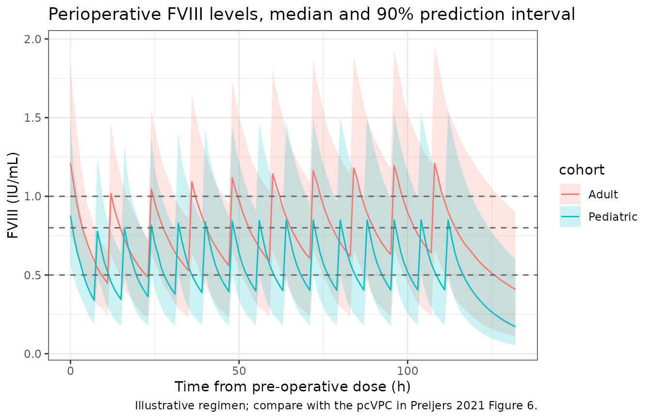
Comparison with the Hazendonk 2016 model
Preijers 2021 Figures 1-2 show that the Hazendonk 2016 model under-predicted typical CL and V1 in young children. The typical 50 IU/kg profiles below compare both models for a one-year-old 10 kg child and a 40-year-old 68 kg adult (non-O, minor surgery, full-length product).
typ_subj <- data.frame(
  id = 1:2, WT = c(10, 68), AGE = c(1, 40), who = c("1 y, 10 kg", "40 y, 68 kg"),
  BLOOD_GROUP_O = 0, SURG_SEV_MAJOR = 0, FORM_FVIII_BDD = 0, FVIIIRECENT = 0,
  STUDY_OPTICLOT_CTR45 = 0, STUDY_GOSH = 0
)
ev_typ <- bind_rows(
  typ_subj |> mutate(time = 0, evid = 1L, amt = 50 * WT, cmt = "central"),
  typ_subj |> tidyr::crossing(time = seq(0, 72, 0.5)) |> mutate(evid = 0L, amt = 0, cmt = "central")
) |>
  arrange(id, time, desc(evid)) |>
  as.data.frame()

typ_both <- bind_rows(
  as.data.frame(rxSolve(zeroRe(mod), ev_typ, keep = "who")) |> mutate(model = "Preijers 2021"),
  as.data.frame(rxSolve(zeroRe(mod_hz), ev_typ, keep = "who")) |> mutate(model = "Hazendonk 2016")
)
#> ℹ parameter labels from comments will be replaced by 'label()'
#> Warning: No sigma parameters in the model
#> ℹ omega/sigma items treated as zero: 'etalcl', 'etalvc'
#> Warning: multi-subject simulation without without 'omega'
#> ℹ parameter labels from comments will be replaced by 'label()'
#> ℹ omega/sigma items treated as zero: 'etalcl', 'etalvc'
#> Warning: multi-subject simulation without without 'omega'

ggplot(typ_both, aes(time, Cc, colour = model)) +
  geom_line() +
  facet_wrap(~who) +
  scale_y_log10() +
  labs(x = "Time after 50 IU/kg (h)", y = "Typical FVIII (IU/mL, log scale)") +
  theme_bw()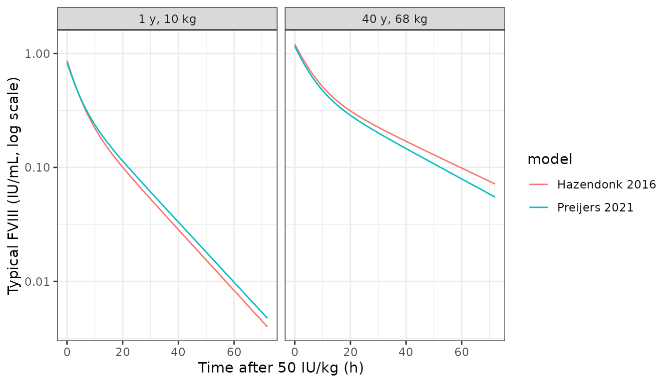
PKNCA validation
nca_in <- sim_single |>
  filter(!is.na(Cc)) |>
  select(id, cohort, time, Cc)
nca_in <- bind_rows(
  nca_in,
  nca_in |> distinct(id, cohort) |> mutate(time = 0, Cc = 0)
) |>
  distinct(id, cohort, time, .keep_all = TRUE) |>
  arrange(id, time)

dose_df <- ev_single |>
  filter(evid == 1) |>
  select(id, cohort, time, amt)

conc_obj <- PKNCAconc(nca_in, Cc ~ time | cohort + id, concu = "IU/mL", timeu = "h")
dose_obj <- PKNCAdose(dose_df, amt ~ time | cohort + id, doseu = "IU", route = "intravascular")
intervals <- data.frame(
  start = 0, end = Inf,
  cmax = TRUE, aucinf.obs = TRUE, half.life = TRUE, cl.obs = TRUE
)
nca_res <- pk.nca(PKNCAdata(conc_obj, dose_obj, intervals = intervals))
knitr::kable(summary(nca_res), caption = "PKNCA summary by cohort, single 50 IU/kg bolus.")| Interval Start | Interval End | cohort | N | Cmax (IU/mL) | Half-life (h) | AUCinf,obs (h*IU/mL) | CL (based on AUCinf,obs) (IU/(h*IU/mL)) |
|---|---|---|---|---|---|---|---|
| 0 | Inf | Adult | 100 | 1.24 [27.7] | 24.4 [5.82] | 21.4 [36.7] | 177 [39.7] |
| 0 | Inf | Pediatric | 100 | 0.893 [25.8] | 13.7 [4.75] | 9.24 [50.6] | 76.0 [54.5] |
The paper reports no NCA, so the NCA is checked against the model
itself: the NCA clearance Dose / AUCinf must recover each
subject’s model clearance (same drawn parameters on both sides, so the
difference is numerical error from the trapezoid rule and the
extrapolated tail).
indiv <- sim_single |>
  distinct(id, cohort, cl, vc, q, vp)
cl_nca <- as.data.frame(nca_res$result) |>
  filter(PPTESTCD == "cl.obs") |>
  select(id, cohort, cl_nca = PPORRES)
chk <- inner_join(indiv, cl_nca, by = c("id", "cohort")) |>
  # cl.obs = IU / (IU/mL * h) is already in mL/h; model cl is in L/h.
  mutate(pct_diff = 100 * (cl_nca / (cl * 1000) - 1))
chk |>
  group_by(cohort) |>
  summarise(
    `median model CL (mL/h)` = round(median(cl * 1000), 1),
    `median NCA CL (mL/h)` = round(median(cl_nca), 1),
    `median % difference` = round(median(pct_diff), 2),
    .groups = "drop"
  ) |>
knitr::kable(caption = "NCA clearance versus model clearance.")| cohort | median model CL (mL/h) | median NCA CL (mL/h) | median % difference |
|---|---|---|---|
| Adult | 169.2 | 169.2 | 0.00 |
| Pediatric | 73.6 | 73.6 | -0.01 |
For the typical 68 kg, 40-year-old adult, the terminal half-life follows from the two-compartment micro-constants:
k10 <- 0.171 / 2.930
k12 <- 0.172 / 2.930
k21 <- 0.172 / 1.810
s <- k10 + k12 + k21
beta <- (s - sqrt(s^2 - 4 * k10 * k21)) / 2
alpha <- (s + sqrt(s^2 - 4 * k10 * k21)) / 2
c(`distribution t1/2 (h)` = log(2) / alpha, `terminal t1/2 (h)` = log(2) / beta)
#> distribution t1/2 (h)     terminal t1/2 (h)
#>               3.81808              22.68964
Endogenous baseline and Refacto AF readout
ro <- data.frame(
  id = 1:3, WT = 68, AGE = 40, BLOOD_GROUP_O = 0,
  FORM_FVIII_BDD = c(0, 0, 1), FVIIIRECENT = c(0, 0.03, 0.03),
  STUDY_OPTICLOT_CTR45 = 0, STUDY_GOSH = 0
)
ev_ro <- bind_rows(
  ro |> mutate(time = 0, evid = 1L, amt = 50 * 68, cmt = "central"),
  ro |> tidyr::crossing(time = c(0, 1, 24)) |> mutate(evid = 0L, amt = 0, cmt = "central")
) |>
  arrange(id, time, desc(evid)) |>
  as.data.frame()
sim_ro <- as.data.frame(rxSolve(zeroRe(mod), ev_ro, keep = c("FVIIIRECENT", "FORM_FVIII_BDD")))
#> ℹ parameter labels from comments will be replaced by 'label()'
#> Warning: No sigma parameters in the model
#> ℹ omega/sigma items treated as zero: 'etalcl', 'etalvc'
#> Warning: multi-subject simulation without without 'omega'
sim_ro |>
  filter(time == 24) |>
  select(FVIIIRECENT, FORM_FVIII_BDD, Cc) |>
knitr::kable(digits = 4, caption = "Typical FVIII 24 h after 50 IU/kg: baseline and BDD-product readout.")| FVIIIRECENT | FORM_FVIII_BDD | Cc |
|---|---|---|
| 0.00 | 0 | 0.2466 |
| 0.03 | 0 | 0.2766 |
| 0.03 | 1 | 0.1936 |
Assumptions and deviations
-
Final model only. The Table 2 ‘Original model’
column is the Hazendonk 2016 model, already available as
Hazendonk_2016_factor_viii; the ‘Structural model’ column is an intermediate step without covariates and is not packaged. The bootstrap medians are not used. -
Methods Eq. 1 read as a multiplicative correction.
As printed, Eq. 1 is
C = (C_PRED + C_base) - theta_prod * (C_PRED + C_base)^theta_RefactoAF, which would subtract a constant 0.30 IU/mL from every non-Refacto sample (anything raised to the power 0 is 1). The text definestheta_prodas “the estimated effect fraction of a FVIII product on the measured FVIII level” andtheta_RefactoAFas a 0/1 indicator, and the Hazendonk 2016 predecessor applied the same correction asC_pred * (1 - theta). The model therefore uses(C_PRED + C_base) * (1 - 0.30 * FORM_FVIII_BDD), which equals(C_PRED + C_base) * (1 - 0.30)^FORM_FVIII_BDDfor a binary indicator. -
Endogenous baseline. Eq. 1 adds the measured
endogenous level
C_baseto the prediction; it is carried as the covariateFVIIIRECENT(IU/mL), the package’s canonical name for the patient’s most recently measured untreated FVIII:C (also used, as a power-scaled covariate, bySchutte_2018_desmopressin). Set it to 0 to simulate the drug-attributable FVIII only. -
Pre-dose FVIII initialisation not encoded. When a
pre-operative FVIII level was available without the preceding dose
history, the authors initialised every compartment at that level times
its volume (NONMEM A_0). This is a data-handling device, not a model
parameter; users can reproduce it by setting
central(0)andperipheral1(0)on the event table. -
IIV variance scale. Table 2 reports IIV as %CV; the
variances are
log(1 + CV^2)(0.1457 and 0.0729). The Hazendonk 2016 model in this package usedCV^2; the two differ by about 7% for CL and less than 1% for V1. -
Centre-specific residual error. All three centre
groups are encoded.
STUDY_OPTICLOT_CTR45 = 1selects centres 4-5 andSTUDY_GOSH = 1selects centre 6 (GOSH); both 0 selects centres 1-3. The paper does not say which Dutch centres are numbered 4 and 5. Table 2 prints the centre 1-3 proportional error as 19.7 (%CV) and the others as fractions (0.21, 0.22); all are used as fractions. - Narrative values not reproduced. Results 3.2 quotes typical CL of 68 mL/h and V1 of 930 mL for a one-year-old 10 kg child under the Hazendonk 2016 model; its equations give 66.7 mL/h and 576 mL. The 930 mL value cannot be recovered from any printed equation, so it is not used.
- Virtual cohort. Weight-for-age knots are approximate medians and the dosing regimen is illustrative; the paper’s individual dosing histories are not published. Sex is taken as all-male (X-linked disease; not tabulated).
- Errata. A Europe PMC search on 2026-09-29 found no correction notice for this article. The supplement (weight imputation model, model-building steps) contains no final parameter values and was not needed.