Burosumab (Lee 2022) • nlmixr2lib

Model and source

Citation: Lee SK, Gosselin NH, Taylor J, Roberts MS, McKeever K, Shi J. Population Pharmacokinetics and Pharmacodynamics of Burosumab in Adult and Pediatric Patients With X-linked Hypophosphatemia. J Clin Pharmacol. 2022;62(1):87-98. doi:10.1002/jcph.1950
Description: One-compartment population PK model with first-order absorption and linear elimination for subcutaneous burosumab (a human anti-FGF23 IgG1 monoclonal antibody) in adult and pediatric (1-12 years) patients with X-linked hypophosphatemia, coupled to a direct Emax model (Hill coefficient fixed to 1) for absolute serum phosphorus. Apparent clearance and volume carry estimated allometric exponents on time-varying body weight referenced to 70 kg, and body weight also scales the baseline serum phosphorus E0 (negative exponent) and the maximal increase Emax (positive exponent).
Article: https://doi.org/10.1002/jcph.1950 (open access)

Lee 2022 pools nine burosumab studies in adults and children with X-linked hypophosphatemia (XLH) and fits two models in sequence: a one-compartment population PK model for serum burosumab, then a direct sigmoid Emax model that links the burosumab concentration to the absolute serum phosphorus. This package encodes both as one model with two outputs: Cc (serum burosumab, ng/mL) and serum_phosphorus (serum phosphorus, mg/dL). The paper’s Supplemental Information 3 gives the Phoenix NLME code of both models, which fixes the equation forms and the residual-error structure.

An earlier analysis of three of the same adult studies is packaged as Zhang_2016_burosumab. That model describes the PD as the change from baseline with an EC50 that drifts upward over time. Lee 2022 replaced it with a time-invariant EC50 on absolute serum phosphorus.

Population

The analysis pooled 277 subjects with XLH from nine clinical studies (Lee 2022 Methods and Table 1). There were 183 adults (>17 years) from six studies and 94 children from three studies: 6 infants aged 1-2 years and 88 children aged 2-12 years. Doses ranged from 0.05 to 1.2 mg/kg subcutaneously, given once or every 2 or 4 weeks, with each subject’s dose titrated on serum phosphorus. The PK analysis used 2844 measurable burosumab concentrations and the PK-PD analysis used 6047 serum phosphorus observations. Across the pooled cohort 59% of subjects were female and 84% White (Table 1); 8.7% were positive for anti-drug antibodies. Baseline serum phosphorus (geometric mean) was 2.6, 2.4 and 2.0 mg/dL in infants, children and adults (Table 2), against a reference range of 2.5-4.5 mg/dL.

The same information is available programmatically via the model’s population metadata (readModelDb("Lee_2022_burosumab")()$population).

Source trace

Equation / parameter	Value	Source location
`lka`	log(0.395) 1/day	Table 3
`lcl`	log(0.297) L/day at 70 kg	Table 3
`lvc`	log(9.02) L at 70 kg	Table 3
`e_wt_cl`	0.912	Table 3, (WT/70) exponent on CL/F
`e_wt_vc`	1.05	Table 3, (WT/70) exponent on V/F
`etalcl`	0.121227 (35.9% CV)	Table 3, BSV column; omega^2 = log(CV^2 + 1)
`etalvc`	0.113694 (34.7% CV)	Table 3, BSV column
BSV on Ka	0% (FIX), no eta	Table 3; absent from the Supplemental Information 3 PK code
`addSd`	32.2 ng/mL	Table 3
`propSd`	0.207	Table 3
`Cc ~ add + prop + combined1()`	SD = a + b * Cc	Supplemental Information 3 PK code, `observe(CObs = C + CEps * (1 + C * CMixRatio))`
`le0`	log(2.03) mg/dL at 70 kg	Table 4
`lec50`	log(4131) ng/mL	Table 4
`lemax`	log(1.59) mg/dL at 70 kg	Table 4
`lhill`	fixed(log(1))	Table 4, Gamma = 1 (FIX); Results ‘Population PK-PD Modeling’
`e_wt_e0`	-0.143	Table 4, (WT/70) exponent on E0
`e_wt_emax`	0.168	Table 4, (WT/70) exponent on Emax
`etale0`	0.014297 (12.0% CV)	Table 4
`etalec50`	0.989541 (130% CV)	Table 4
`etalemax`	0.249220 (53.2% CV)	Table 4
`propSd_serum_phosphorus`	0.132	Table 4; Supplemental Information 3 PK-PD code `observe(EObs = E * (1 + EEps))`
`d/dt(depot)`, `d/dt(central)`	first-order absorption, linear elimination	Results ‘Population PK Modeling’; Supplemental Information 3 `deriv()` lines
`serum_phosphorus <- e0 + emax * Cc^hill / (ec50^hill + Cc^hill)`	n/a	Supplemental Information 3 PK-PD code, `E = E0 + Emax * C^Gam / (EC50^Gam + C^Gam)`
`(WT / 70)` power terms on CL/F, V/F, E0, Emax	time-varying WT, reference 70 kg	Table 3 and Table 4 footnotes

Typical-value checks

These checks use the published typical values directly, so they are exact and do not depend on a simulated cohort.

The Discussion quotes a typical elimination half-life of 16 to 19 days across adults and children. With the Table 3 values the half-life, log(2) * V/F / (CL/F), depends on body weight only through WT^(1.05 - 0.912):

mod <- readModelDb("Lee_2022_burosumab")
ui <- rxode2::rxode(mod)
#> ℹ parameter labels from comments will be replaced by 'label()'
th <- ui$theta
thalf <- function(wt) {
  cl <- exp(th[["lcl"]]) * (wt / 70)^th[["e_wt_cl"]]
  vc <- exp(th[["lvc"]]) * (wt / 70)^th[["e_wt_vc"]]
  log(2) * vc / cl
}
hl <- data.frame(WT = c(8, 15, 30, 50, 70, 100))
hl$thalf <- thalf(hl$WT)
hl |>
  dplyr::rename("Body weight (kg)" = WT, "Typical t1/2 (day)" = thalf) |>
  knitr::kable(digits = 1, caption = "Typical elimination half-life by body weight.")

Typical elimination half-life by body weight.
Body weight (kg)	Typical t1/2 (day)
8	15.6
15	17.0
30	18.7
50	20.1
70	21.1
100	22.1

stopifnot(
  # Closed form from Table 3: 0.693 * 9.02 / 0.297 = 21.05 days at 70 kg.
  abs(thalf(70) - 21.05) < 0.01
)

The 16-19 day range in the Discussion is reproduced for children from about 10 to 35 kg. The typical 70-kg adult value from Table 3 is 21 days, and the paper does not say how its adult figure was derived (see Assumptions and deviations).

At steady state, the AUC over a dosing interval of a linear model is dose / (CL/F). For a 70-kg adult on 1 mg/kg every 4 weeks this is 70 / 0.297 = 236 ug*day/mL, in line with the median of about 235 ug*day/mL in the Supplemental Information 9 box plot.

Virtual cohorts

The observed data are not public. The simulations below follow the paper’s own simulation scenarios. Each arm has 200 subjects:

Adolescents, 0.8 mg/kg every 2 weeks (Q2W) – Supplemental Information 6. The paper drew adolescent weights from a GAMLSS model fitted to the study cohort; that fit is not published. Here ages are uniform on 12-17 years and weights are log-normal (SD 0.2 on the log scale) around a growth-chart median for each age.
Children 1-5 years, 0.8 mg/kg Q2W and infants 6-10 kg, 1 mg/kg Q2W – Supplemental Information 7. The infant weight range is the paper’s (5th to 95th percentile at 6 months on the CDC charts), sampled uniformly.
Adults, 1 mg/kg every 4 weeks (Q4W), and adults, 70 mg flat dose Q4W – Supplemental Information 9. Adult weights are log-normal with median 72 kg and SD 0.22 on the log scale.
Adult dose escalation, Q4W 0.3 -> 0.5 -> 1 -> 1 mg/kg and pediatric dose escalation, Q2W 0.4 -> 1 -> 2 -> 2 mg/kg – Supplemental Information
1. The pediatric cohort spans ages 1-12 years.

Body weight is held constant within each subject over the simulation. The steady-state arms take 26 doses (Q2W) or 13 doses (Q4W), about 17 typical half-lives, and are read out over the last dosing interval.

# rxSetSeed() makes the draw reproducible on a given machine. rxode2's random
# streams are split per solver thread, so another thread count draws a
# different cohort. The assertions below therefore use medians and wide
# tolerances, not extremes (see the comments next to each bound).
rxode2::rxSetSeed(20220101)
set.seed(20220101)
n_arm <- 200

# Approximate growth-chart median weight (kg) by age, sexes pooled.
wt_age <- data.frame(
  age = c(1, 2, 3, 4, 5, 6, 8, 10, 12, 13, 14, 15, 16, 17),
  wt = c(9.6, 12.2, 14.3, 16.3, 18.3, 20.5, 25.6, 31.9, 40.5, 45.5, 50.5, 55, 58.5, 61.5)
)
median_wt <- function(age) stats::approx(wt_age$age, wt_age$wt, xout = age)$y

cohort <- dplyr::bind_rows(
  data.frame(arm = "Adolescents 0.8 mg/kg Q2W", WT = median_wt(runif(n_arm, 12, 17)) * exp(rnorm(n_arm, 0, 0.2))),
  data.frame(arm = "Children 1-5 y 0.8 mg/kg Q2W", WT = median_wt(runif(n_arm, 1, 5)) * exp(rnorm(n_arm, 0, 0.13))),
  data.frame(arm = "Infants 1 mg/kg Q2W", WT = runif(n_arm, 6, 10)),
  data.frame(arm = "Adults 1 mg/kg Q4W", WT = exp(rnorm(n_arm, log(72), 0.22))),
  data.frame(arm = "Adults 70 mg Q4W", WT = exp(rnorm(n_arm, log(72), 0.22))),
  data.frame(arm = "Adult escalation Q4W", WT = exp(rnorm(n_arm, log(72), 0.22))),
  data.frame(arm = "Pediatric escalation Q2W", WT = median_wt(runif(n_arm, 1, 12)) * exp(rnorm(n_arm, 0, 0.13)))
)
cohort$id <- seq_len(nrow(cohort))

arm_design <- list(
  "Adolescents 0.8 mg/kg Q2W" = list(tau = 14, mgkg = rep(0.8, 26)),
  "Children 1-5 y 0.8 mg/kg Q2W" = list(tau = 14, mgkg = rep(0.8, 26)),
  "Infants 1 mg/kg Q2W" = list(tau = 14, mgkg = rep(1, 26)),
  "Adults 1 mg/kg Q4W" = list(tau = 28, mgkg = rep(1, 13)),
  "Adults 70 mg Q4W" = list(tau = 28, flat = 70, n = 13),
  "Adult escalation Q4W" = list(tau = 28, mgkg = c(0.3, 0.5, 1, 1)),
  "Pediatric escalation Q2W" = list(tau = 14, mgkg = c(0.4, 1, 2, 2))
)

make_events <- function(id, arm, wt) {
  des <- arm_design[[arm]]
  amt <- if (!is.null(des$flat)) rep(des$flat, des$n) else des$mgkg * wt
  nd <- length(amt)
  dose_t <- (seq_len(nd) - 1) * des$tau
  if (grepl("escalation", arm)) {
    obs_t <- seq(0, nd * des$tau, by = 0.5)
  } else {
    # time 0 plus a dense grid over the final dosing interval
    obs_t <- c(0, seq(dose_t[nd], dose_t[nd] + des$tau, by = 0.25))
  }
  dplyr::bind_rows(
    data.frame(id = id, time = dose_t, amt = amt, evid = 1L, cmt = "depot", dvid = NA_integer_),
    data.frame(id = id, time = obs_t, amt = 0, evid = 0L, cmt = NA_character_, dvid = 1L)
  ) |>
    dplyr::mutate(arm = arm, WT = wt)
}

events <- dplyr::bind_rows(lapply(seq_len(nrow(cohort)), function(i) {
  make_events(cohort$id[i], cohort$arm[i], cohort$WT[i])
})) |>
  dplyr::arrange(id, time, dplyr::desc(evid))

cohort |>
  dplyr::group_by(arm) |>
  dplyr::summarise(
    n = dplyr::n(),
    `Median WT (kg)` = median(WT),
    `5th pct WT` = quantile(WT, 0.05),
    `95th pct WT` = quantile(WT, 0.95),
    .groups = "drop"
  ) |>
  dplyr::rename(Arm = arm) |>
  knitr::kable(digits = 1, caption = "Virtual cohorts.")

Virtual cohorts.
Arm	n	Median WT (kg)	5th pct WT	95th pct WT
Adolescents 0.8 mg/kg Q2W	200	52.3	34.2	76.9
Adult escalation Q4W	200	74.7	49.9	102.1
Adults 1 mg/kg Q4W	200	73.6	51.4	102.0
Adults 70 mg Q4W	200	70.7	51.4	96.8
Children 1-5 y 0.8 mg/kg Q2W	200	14.4	10.1	19.3
Infants 1 mg/kg Q2W	200	8.0	6.3	9.8
Pediatric escalation Q2W	200	19.6	9.6	38.1

The model has two outputs (Cc and serum_phosphorus), so observation rows carry dvid = 1 and no cmt; the solve still returns both outputs on every observation row.

sim <- rxode2::rxSolve(mod, events, keep = c("arm", "WT"), returnType = "data.frame")
#> ℹ parameter labels from comments will be replaced by 'label()'
stopifnot(!anyNA(sim$Cc), !anyNA(sim$serum_phosphorus))

Steady-state PK: PKNCA

NCA runs over the final dosing interval of each steady-state arm.

ss_arms <- c(
  "Adolescents 0.8 mg/kg Q2W", "Children 1-5 y 0.8 mg/kg Q2W",
  "Infants 1 mg/kg Q2W", "Adults 1 mg/kg Q4W", "Adults 70 mg Q4W"
)
ss_start <- vapply(ss_arms, function(a) {
  d <- arm_design[[a]]
  (if (is.null(d$n)) length(d$mgkg) else d$n) * d$tau - d$tau
}, numeric(1))
ss_tau <- vapply(ss_arms, function(a) arm_design[[a]]$tau, numeric(1))

conc_df <- sim |>
  dplyr::filter(arm %in% ss_arms, !is.na(Cc)) |>
  dplyr::select(id, time, Cc, treatment = arm)
dose_df <- events |>
  dplyr::filter(arm %in% ss_arms, evid == 1) |>
  dplyr::select(id, time, amt, treatment = arm)

intervals <- data.frame(
  treatment = ss_arms,
  start = ss_start,
  end = ss_start + ss_tau,
  cmax = TRUE,
  cmin = TRUE,
  cav = TRUE,
  auclast = TRUE
)

conc_obj <- PKNCA::PKNCAconc(conc_df, Cc ~ time | treatment + id, concu = "ng/mL", timeu = "day")
dose_obj <- PKNCA::PKNCAdose(dose_df, amt ~ time | treatment + id, doseu = "mg")
nca_res <- PKNCA::pk.nca(PKNCA::PKNCAdata(conc_obj, dose_obj, intervals = intervals))

The published values are medians of 1000 virtual subjects. Supplemental Information 6 and 7 print them. The Supplemental Information 9 values were read off the box plot by the maintainers, so they are approximate. AUC is printed in ugday/mL and is converted to ngday/mL here.

published <- tibble::tribble(
  ~treatment,                     ~cmin, ~cav,  ~cmax, ~auclast,
  "Adolescents 0.8 mg/kg Q2W",    9691,  12388, 14287, NA,
  "Children 1-5 y 0.8 mg/kg Q2W", NA,    NA,    NA,    171000,
  "Infants 1 mg/kg Q2W",          NA,    NA,    NA,    191000,
  "Adults 1 mg/kg Q4W",           5300,  NA,    10800, 235000,
  "Adults 70 mg Q4W",             5300,  NA,    11000, 235000
)

cmp <- nlmixr2lib::ncaComparisonTable(
  simulated = nca_res,
  reference = published,
  by = "treatment",
  units = c(cmin = "ng/mL", cav = "ng/mL", cmax = "ng/mL", auclast = "ng*day/mL"),
  tolerance_pct = 20
)
knitr::kable(
  cmp,
  caption = paste(
    "Simulated vs published steady-state exposure (medians).",
    "* marks a difference above 20%."
  )
)

Simulated vs published steady-state exposure (medians). * marks a difference above 20%.
NCA parameter	treatment	Reference	Simulated	% diff
Cmax (ng/mL)	Adolescents 0.8 mg/kg Q2W	14300	14800	+3.8%
Cmax (ng/mL)	Children 1-5 y 0.8 mg/kg Q2W	—	13800	—
Cmax (ng/mL)	Infants 1 mg/kg Q2W	—	15600	—
Cmax (ng/mL)	Adults 1 mg/kg Q4W	10800	10700	-0.7%
Cmax (ng/mL)	Adults 70 mg Q4W	11000	10700	-2.5%
Cmin (ng/mL)	Adolescents 0.8 mg/kg Q2W	9690	11200	+15.3%
Cmin (ng/mL)	Children 1-5 y 0.8 mg/kg Q2W	—	9960	—
Cmin (ng/mL)	Infants 1 mg/kg Q2W	—	10600	—
Cmin (ng/mL)	Adults 1 mg/kg Q4W	5300	5660	+6.8%
Cmin (ng/mL)	Adults 70 mg Q4W	5300	5440	+2.6%
AUClast (ng*day/mL)	Adolescents 0.8 mg/kg Q2W	—	188000	—
AUClast (ng*day/mL)	Children 1-5 y 0.8 mg/kg Q2W	171000	168000	-2.0%
AUClast (ng*day/mL)	Infants 1 mg/kg Q2W	191000	190000	-0.6%
AUClast (ng*day/mL)	Adults 1 mg/kg Q4W	235000	236000	+0.2%
AUClast (ng*day/mL)	Adults 70 mg Q4W	235000	231000	-1.6%
Cavg (ng/mL)	Adolescents 0.8 mg/kg Q2W	12400	13400	+8.3%
Cavg (ng/mL)	Children 1-5 y 0.8 mg/kg Q2W	—	12000	—
Cavg (ng/mL)	Infants 1 mg/kg Q2W	—	13600	—
Cavg (ng/mL)	Adults 1 mg/kg Q4W	—	8410	—
Cavg (ng/mL)	Adults 70 mg Q4W	—	8260	—


nca_med <- as.data.frame(nca_res$result) |>
  dplyr::group_by(treatment, PPTESTCD) |>
  dplyr::summarise(med = median(PPORRES), .groups = "drop")
pub_long <- published |>
  tidyr::pivot_longer(-treatment, names_to = "PPTESTCD", values_to = "ref") |>
  dplyr::filter(!is.na(ref))
chk <- dplyr::inner_join(nca_med, pub_long, by = c("treatment", "PPTESTCD")) |>
  dplyr::mutate(pct = 100 * (med - ref) / ref)
ado_cmin <- chk$treatment == "Adolescents 0.8 mg/kg Q2W" & chk$PPTESTCD == "cmin"
stopifnot(
  nrow(chk) == 11,
  # Medians of a mg/kg-dosed linear model sit close to the typical value, so
  # a wrong CL/F, V/F, unit or exponent moves them by tens of percent. The
  # other ten medians are within about 8%.
  all(abs(chk$pct[!ado_cmin]) < 15),
  abs(median(chk$pct)) < 8,
  # Known deviation: the adolescent Cmin runs 12-15% high (see the text
  # below), so it gets a looser bound of its own.
  abs(chk$pct[ado_cmin]) < 30
)

Apart from the adolescent Cmin, the medians agree within about 8%. The adolescent Cmin is about 15% above the published 9691 ng/mL (12% in a 1000-subject run). The simulated Cmax/Cmin ratio for that arm is about 1.3, while the published medians imply 1.47, so the published simulation shows a larger peak-to-trough swing than the Table 3 parameters produce at steady state. Supplemental Information 6 also prints 5th-95th percentile ranges (e.g. Cavg 2258-66180 ng/mL) that are far wider than the 35.9% CV on CL/F allows: Cavg at steady state depends only on CL/F, and that variability implies roughly a 3.3-fold 90% range, not a 29-fold one. Those ranges are not reproduced and are not used as a check.

Steady-state serum phosphorus

pd_ss <- sim |>
  dplyr::filter(arm %in% ss_arms) |>
  dplyr::left_join(
    data.frame(arm = ss_arms, start = ss_start, tau = ss_tau),
    by = "arm"
  ) |>
  dplyr::filter(time >= start) |>
  dplyr::group_by(arm, id) |>
  dplyr::summarise(
    phos_min = min(serum_phosphorus),
    phos_max = max(serum_phosphorus),
    phos_avg = sum(diff(time) * (head(serum_phosphorus, -1) + tail(serum_phosphorus, -1)) / 2) / tau[1],
    .groups = "drop"
  ) |>
  tidyr::pivot_longer(dplyr::starts_with("phos_"), names_to = "metric", values_to = "value") |>
  dplyr::group_by(arm, metric) |>
  dplyr::summarise(sim = median(value), .groups = "drop")

pd_pub <- tibble::tribble(
  ~arm,                           ~metric,    ~published,
  "Adolescents 0.8 mg/kg Q2W",    "phos_min", 3.18,
  "Adolescents 0.8 mg/kg Q2W",    "phos_avg", 3.29,
  "Adolescents 0.8 mg/kg Q2W",    "phos_max", 3.34,
  "Children 1-5 y 0.8 mg/kg Q2W", "phos_avg", 3.43,
  "Infants 1 mg/kg Q2W",          "phos_avg", 3.59,
  "Adults 1 mg/kg Q4W",           "phos_min", 2.85,
  "Adults 1 mg/kg Q4W",           "phos_avg", 3.00,
  "Adults 1 mg/kg Q4W",           "phos_max", 3.10
)
pd_chk <- dplyr::inner_join(pd_pub, pd_ss, by = c("arm", "metric")) |>
  dplyr::mutate(diff = sim - published)

pd_chk |>
  dplyr::mutate(metric = dplyr::recode(metric, phos_min = "Cmin", phos_avg = "Cavg", phos_max = "Cmax")) |>
  dplyr::rename(Arm = arm, `Serum phosphorus` = metric, `Published (mg/dL)` = published,
                `Simulated median (mg/dL)` = sim, `Difference (mg/dL)` = diff) |>
  knitr::kable(digits = 2, caption = paste(
    "Steady-state serum phosphorus: simulated medians vs Supplemental",
    "Information 6 and 7 (printed) and 9 (read from the box plot)."
  ))

Steady-state serum phosphorus: simulated medians vs Supplemental Information 6 and 7 (printed) and 9 (read from the box plot).
Arm	Serum phosphorus	Published (mg/dL)	Simulated median (mg/dL)	Difference (mg/dL)
Adolescents 0.8 mg/kg Q2W	Cmin	3.18	3.22	0.04
Adolescents 0.8 mg/kg Q2W	Cavg	3.29	3.29	0.00
Adolescents 0.8 mg/kg Q2W	Cmax	3.34	3.33	-0.01
Children 1-5 y 0.8 mg/kg Q2W	Cavg	3.43	3.48	0.05
Infants 1 mg/kg Q2W	Cavg	3.59	3.61	0.02
Adults 1 mg/kg Q4W	Cmin	2.85	2.78	-0.07
Adults 1 mg/kg Q4W	Cavg	3.00	3.00	0.00
Adults 1 mg/kg Q4W	Cmax	3.10	3.12	0.02


stopifnot(
  # E0 and Emax enter additively, so a mis-transcribed E0, Emax, EC50 or WT
  # exponent shifts these medians by 0.3 mg/dL or more. The realised
  # differences are within about 0.1 mg/dL.
  all(abs(pd_chk$diff) < 0.25),
  abs(median(pd_chk$diff)) < 0.12
)

Dose escalation (Supplemental Information 8)

Supplemental Information 8 simulates a forced dose escalation and prints the percentage of subjects whose trough serum phosphorus is above the lower limit of normal at the end of each dosing interval. That limit is 2.5 mg/dL in adults and 3.2 mg/dL in children. Figure 1 below repeats the adult panel and Figure 2 the pediatric panel.

esc <- sim |>
  dplyr::filter(grepl("escalation", arm)) |>
  dplyr::group_by(arm, time) |>
  dplyr::summarise(
    dplyr::across(c(Cc, serum_phosphorus), list(
      p05 = ~ quantile(.x, 0.05), p25 = ~ quantile(.x, 0.25),
      p50 = median, p75 = ~ quantile(.x, 0.75), p95 = ~ quantile(.x, 0.95)
    )),
    .groups = "drop"
  ) |>
  tidyr::pivot_longer(-c(arm, time), names_to = c("output", ".value"), names_pattern = "(Cc|serum_phosphorus)_(p..)") |>
  dplyr::mutate(output = dplyr::recode(output, Cc = "Burosumab (ng/mL)", serum_phosphorus = "Serum phosphorus (mg/dL)"))

lln <- data.frame(
  arm = c("Adult escalation Q4W", "Pediatric escalation Q2W"),
  output = "Serum phosphorus (mg/dL)",
  y = c(2.5, 3.2)
)

ggplot(esc, aes(time / 7, p50)) +
  geom_ribbon(aes(ymin = p05, ymax = p95), fill = "grey85") +
  geom_ribbon(aes(ymin = p25, ymax = p75), fill = "grey65") +
  geom_line() +
  geom_hline(data = lln, aes(yintercept = y), colour = "red") +
  facet_grid(output ~ arm, scales = "free") +
  labs(
    x = "Time after first dose (weeks)", y = NULL,
    caption = paste(
      "Median, 50% and 90% prediction intervals; red line = lower limit of normal.",
      "Replicates Supplemental Information 8a (adults) and 8b (pediatrics) of Lee 2022."
    )
  ) +
  theme_bw()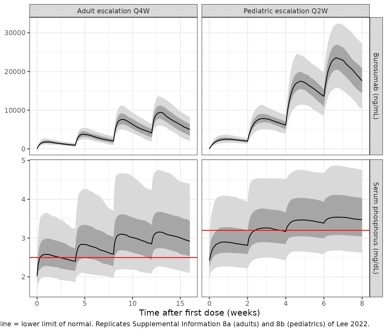

trough_t <- function(arm) {
  d <- arm_design[[arm]]
  seq_along(d$mgkg) * d$tau
}
esc_pub <- dplyr::bind_rows(
  data.frame(arm = "Adult escalation Q4W", time = trough_t("Adult escalation Q4W"),
             dose = c("0.3 mg/kg", "0.5 mg/kg", "1 mg/kg", "1 mg/kg"),
             lln = 2.5, published = c(33.6, 54.8, 73.9, 77.3)),
  data.frame(arm = "Pediatric escalation Q2W", time = trough_t("Pediatric escalation Q2W"),
             dose = c("0.4 mg/kg", "1 mg/kg", "2 mg/kg", "2 mg/kg"),
             lln = 3.2, published = c(16.7, 39.7, 60.3, 67.8))
)
# The observation grid lands exactly on each trough time. A dose given at the
# same time enters the depot, so it does not change Cc or serum_phosphorus at that instant.
esc_sim <- sim |>
  dplyr::inner_join(esc_pub, by = c("arm", "time")) |>
  dplyr::group_by(arm, time, dose, published) |>
  dplyr::summarise(
    simulated = 100 * mean(serum_phosphorus > lln),
    median_trough_Cc = median(Cc),
    .groups = "drop"
  ) |>
  dplyr::mutate(diff = simulated - published)

esc_sim |>
  dplyr::rename(Arm = arm, `Trough (day)` = time, Dose = dose,
                `Published % above LLN` = published, `Simulated % above LLN` = simulated,
                `Median trough burosumab (ng/mL)` = median_trough_Cc,
                `Difference (points)` = diff) |>
  knitr::kable(digits = 1, caption = "Percentage of troughs above the lower limit of normal (LLN).")

Percentage of troughs above the lower limit of normal (LLN).
Arm	Trough (day)	Dose	Published % above LLN	Simulated % above LLN	Median trough burosumab (ng/mL)	Difference (points)
Adult escalation Q4W	28	0.3 mg/kg	33.6	42.5	944.7	8.9
Adult escalation Q4W	56	0.5 mg/kg	54.8	56.0	2034.3	1.2
Adult escalation Q4W	84	1 mg/kg	73.9	73.0	4093.4	-0.9
Adult escalation Q4W	112	1 mg/kg	77.3	75.5	5040.9	-1.8
Pediatric escalation Q2W	14	0.4 mg/kg	16.7	25.5	1993.3	8.8
Pediatric escalation Q2W	28	1 mg/kg	39.7	49.0	6144.9	9.3
Pediatric escalation Q2W	42	2 mg/kg	60.3	63.0	13581.9	2.7
Pediatric escalation Q2W	56	2 mg/kg	67.8	67.5	17629.1	-0.3


adult_esc <- dplyr::filter(esc_sim, arm == "Adult escalation Q4W")
ped_esc <- dplyr::filter(esc_sim, arm == "Pediatric escalation Q2W")
stopifnot(
  # With 200 subjects a percentage has a Monte-Carlo SE of about 3.5 points.
  # The adult differences were 2-3 points in 1000-subject runs and up to 9
  # points at 200 subjects; 15 still catches a wrong EC50 or E0. The first two
  # pediatric steps are a known deviation (see below), so only the last two
  # pediatric steps are checked.
  all(abs(adult_esc$diff) < 15),
  all(abs(ped_esc$diff[3:4]) < 15),
  # Trend over the escalation, not step-by-step ordering.
  adult_esc$simulated[4] > adult_esc$simulated[1] + 20,
  ped_esc$simulated[4] > ped_esc$simulated[1] + 20
)

The model reproduces the adult panel. In 1000-subject runs each adult step is within 2-3 points of the figure; at 200 subjects the first step can be up to about 9 points off by chance. The median burosumab troughs in both panels also match the figure: about 950, 2000, 4000 and 4900 ng/mL in adults, and about 2000, 6100, 13600 and 18000 ng/mL in children. In the pediatric panel the last two steps match, but at the first two steps (0.4 and 1 mg/kg) about 10 points more simulated children are above 3.2 mg/dL than the figure shows. Because the PK troughs agree, the difference is in the pediatric phosphorus response at low concentrations. In this model that response depends mainly on the virtual children’s body weights, through E0 and Emax. The paper does not describe the age or weight make-up of its pediatric virtual population.

Assumptions and deviations

BSV scale. Tables 3 and 4 report BSV as a percentage on log-normally distributed parameters, without naming the conversion. Variances are encoded as omega^2 = log(CV^2 + 1). The alternative omega^2 = CV^2 matters mostly for EC50 (0.99 vs 1.69). The maintainers simulated the Supplemental Information 7 and 8 scenarios under both readings. The two were close, and log(CV^2 + 1) matched the adult escalation percentages slightly better.
No random-effect correlations. The Supplemental Information 3 code declares block(nV, nCl) and block(nE0, nEmax, nEC50) with round starting values. The paper states the PK BSV was modelled without correlation and that the PK-PD BSV followed the same approach, and no covariance is tabulated. The model therefore uses a diagonal omega.
Supplemental code is not the final model. The PK-PD code in Supplemental Information 3 still carries baseline FGF23, alkaline phosphatase and study-design terms, and no body-weight effect on Emax. These were tested and removed; the final model in Table 4 keeps only WT on E0 and Emax. The code is used only for the equation forms and the residual-error structure.
PK residual error. Phoenix’s C + CEps * (1 + C * CMixRatio) makes the residual SD a linear sum a + b * C, which is nlmixr2’s combined1(). Table 3’s 20.7% is read as the proportional SD b. The code’s starting values support this reading: 32.464 * 0.00675 = 0.219, close to 0.207.
Sequential vs joint fit. The authors fitted the PK-PD model on individual PK predictions. Here the PD is driven by the model’s own Cc, which gives the same predictions for a given set of PK parameters.
Absorption. Table 3 fixes the BSV on Ka at 0%, and the model has no Ka eta.
Half-life. The Discussion’s typical half-life of 16-19 days in adults and children is reproduced only for children (about 10-35 kg); Table 3 gives 21 days at 70 kg.
Adolescent exposure. The GAMLSS weight model used for the adolescents is not published, so adolescent weights come from growth-chart medians. The wide 5th-95th percentile ranges in Supplemental Information 6 cannot be reproduced from the published variability.
Discussion vs Supplemental Information 8. The Discussion quotes 12.7% to 67.0% of children reaching normal trough phosphorus “when burosumab dose escalated from 0.3 mg/kg up to 2.0 mg/kg” and about 36% at 0.8 mg/kg Q2W. The scheme behind those numbers is not described. The Supplemental Information 8b figure, which starts at 0.4 mg/kg, is the one reproduced here.
Dose units. Doses are in mg and V/F is in L, so Cc = 1000 * central / vc gives ng/mL, the unit of the assay, the additive residual error and EC50.