Talazoparib + enzalutamide combination therapy (Hadigol 2026) • nlmixr2lib

Model and source

#> ℹ parameter labels from comments will be replaced by 'label()'

Citation: Hadigol M, Williams JH, Shi H, Yang DZ, Hoffman J, Wang DD. Population Pharmacokinetics Analysis of Talazoparib and Enzalutamide Combination Therapy for Patients With Metastatic Castration-Resistant Prostate Cancer. J Clin Pharmacol. 2026;66(2):e70125. doi:10.1002/jcph.70125.
Article: https://doi.org/10.1002/jcph.70125
Trial: TALAPRO-2, https://clinicaltrials.gov/study/NCT03395197

This vignette validates a single model file that carries three coupled analytes: talazoparib, enzalutamide, and the active metabolite N-desmethyl enzalutamide. The three cannot be separated into independent models, because talazoparib’s apparent clearance is a function of the instantaneous plasma concentration of the other two – simulating talazoparib requires simulating the enzalutamide sub-system alongside it.

Population

The model was fit to 811 men with metastatic castration-resistant prostate cancer (mCRPC), pooled from Part 1 (19 patients, open-label, non-randomized, dense sampling) and Part 2 Cohort 1 (792 patients, randomized, double-blind, sparse sampling) of the Phase 3 TALAPRO-2 trial. Part 2 Cohort 1 enrolled patients unselected for homologous recombination repair (HRR) gene deficiencies; the HRR-deficient Cohort 2 was not pooled into this analysis.

414 patients were randomized to talazoparib plus enzalutamide and 397 to placebo plus enzalutamide, so all 811 contribute enzalutamide and N-desmethyl enzalutamide data while only the 412 of 414 with at least one non-BLQ talazoparib observation contribute talazoparib data. The dataset comprised 6030 plasma observations for enzalutamide and for N-desmethyl enzalutamide, and 2961 for talazoparib.

Enzalutamide was dosed at 160 mg once daily with protocol-permitted reductions to 120 mg and 80 mg. Talazoparib was dosed at 0.5 mg once daily, reduced to a 0.35 mg once-daily starting dose in moderate renal impairment. Part 1 initially combined talazoparib 1 mg once daily with enzalutamide, which produced roughly two-fold higher than expected talazoparib troughs at Week 5 along with more Grade 3/4 haematologic adverse events than expected; that is the observation the drug-drug interaction term in this model quantifies, and the reason the combination dose is 0.5 mg rather than 1 mg.

The medians named in the main text are baseline body weight 80.1 kg and age 71 years (both stated as population medians), with 86.85 mL/min the baseline creatinine clearance of the typical patient used as the reference in the covariate equation. Tables S1 and S2 (study-population summary and baseline demographics) are not open access, so covariate ranges and the race/ethnicity and regional breakdown cannot be recorded here – see “Assumptions and deviations”.

The same information is available programmatically via the model’s population metadata (readModelDb("Hadigol_2026_talazoparib_enzalutamide")()$population).

Model structure

Hadigol 2026 Figure 1 gives the enzalutamide parent-metabolite schematic; the talazoparib arm is described in the Drug-Drug Interactions section. The packaged model reproduces all three:

Enzalutamide (suffix _enz) is absorbed first-order from depot_enz into central_enz, distributes to peripheral1_enz, and leaves central_enz at the full apparent clearance CLe/Fe. A fraction Fmet of that flux is routed into the metabolite; the remaining (1 - Fmet) is true elimination. Writing it this way keeps total enzalutamide apparent clearance equal to CLe/Fe for any value of Fmet – which is exactly why Fmet and the metabolite volume Vcn are not simultaneously identifiable from parent and metabolite plasma data alone. Hadigol 2026 resolved this by fixing Fmet to 0.634 from a published enzalutamide PBPK model, having found that fit better than the alternative literature device of assuming equal central volumes for parent and metabolite.

N-desmethyl enzalutamide (suffix _ndmenz) is two-compartment with no depot: it is formed directly into plasma.

Talazoparib carries the bare canonical names, because it is the substrate of interest. It is two-compartment with first-order absorption and – unlike the talazoparib monotherapy model – no absorption lag time. Its apparent clearance is built in two stages: equation (6) applies the renal-function power effect to give the interaction-free base clearance CLt0/Ft, then equation (1) applies the P-glycoprotein inhibition term

$\mathrm{CL}_t/F_t = \mathrm{CL}_{t0}/F_t \times \bigl(1 - \theta_{slope} \times (C_e + C_n)\bigr)$

so the clearance is time-varying, tracking the perpetrator concentrations through the dosing interval. The two perpetrator species enter with equal weight because Hadigol 2026 considered them equipotent on the basis of in vitro data. When the enzalutamide depot is never dosed, both perpetrator compartments stay at zero, the bracket evaluates to exactly 1, and talazoparib clearance falls back to its uninhibited base value.

The three sub-models were fit sequentially (enzalutamide; then the metabolite with enzalutamide parameters fixed to empirical Bayes estimates; then talazoparib with both fixed), because a simultaneous parent-metabolite fit was not stable. There is therefore no cross-analyte random-effect covariance to carry, and the packaged model has three separate variability blocks.

Source trace

Every ini() entry in inst/modeldb/specificDrugs/Hadigol_2026_talazoparib_enzalutamide.R carries an in-file comment naming its source row, together with the reported SE, RSE and the PsN sampling-importance-resampling median and 95% CI. The table below collects them.

Source trace. Table numbers are Hadigol 2026 main-text tables; equation numbers are its numbered display equations.
Analyte	Parameter	Value	Source
Talazoparib	`lcl` (CLt0/Ft)	5.078 L/h	Table 3
Talazoparib	`lvc` (Vct/Ft)	14.389 L	Table 3
Talazoparib	`lvp` (Vpt/Ft)	382.135 L	Table 3
Talazoparib	`lq` (Qt/Ft)	15.568 L/h	Table 3
Talazoparib	`lka` (kat)	0.157 1/h	Table 3
Talazoparib	`lfdepot` (Ft)	1 (fixed)	Table 3
Talazoparib	`e_crcl_cl`	0.455	Table 3 + equation (6)
Talazoparib	`e_cenz_cl` (theta slope)	6.58e-6 mL/ng	Table 3 + equation (1)
Talazoparib	`etalcl`, `etalvc`	0.073, 2.582	Table 3 (variances)
Talazoparib	`expSd`	0.354	Table 3 ‘Thetarized sigma’
Enzalutamide	`lcl_enz` (CLe/Fe)	0.425 L/h	Table 1
Enzalutamide	`lvc_enz` (Vce/Fe)	25.293 L	Table 1
Enzalutamide	`lvp_enz` (Vpe/Fe)	45.928 L	Table 1
Enzalutamide	`lq_enz` (Qe/Fe)	20.644 L/h	Table 1
Enzalutamide	`lka_enz` (kae)	3.431 1/h	Table 1
Enzalutamide	`lfdepot_enz` (Fe)	1 (fixed)	Table 1
Enzalutamide	`e_wt_cl_enz`	0.549 (power)	Table 1 + equation (2)
Enzalutamide	`e_age_cl_enz`	-0.003 (linear)	Table 1 + equation (2)
Enzalutamide	`e_wt_vc_enz`	3.495 (power)	Table 1 + equation (3)
Enzalutamide	`e_age_vc_enz`	1.223 (power)	Table 1 + equation (3)
Enzalutamide	`etalcl_enz`+`etalvc_enz`	0.037, -0.015, 0.350	Table 1 block Omega
Enzalutamide	`expSd_enz`	0.145	Table 1 ‘Thetarized sigma’
N-desmethyl	`lcl_ndmenz` (CLn)	0.286 L/h	Table 2
N-desmethyl	`lvc_ndmenz` (Vcn)	44.944 L	Table 2
N-desmethyl	`lvp_ndmenz` (Vpn)	52.373 L	Table 2
N-desmethyl	`lq_ndmenz` (Qn)	9.443 L/h	Table 2
N-desmethyl	`fm` (Fmet)	0.634 (fixed)	Table 2; fixed from a published enzalutamide PBPK model
N-desmethyl	`e_wt_cl_ndmenz`	0.006 (linear)	Table 2 + equation (4)
N-desmethyl	`e_wt_vc_ndmenz`	0.027 (linear)	Table 2 + equation (5)
N-desmethyl	`etalcl_ndmenz`+`etalvc_ndmenz`	0.057, 0.006, 0.342	Table 2 block Omega
N-desmethyl	`expSd_ndmenz`	0.125	Table 2 ‘Thetarized sigma’

Typical-value simulation machinery

Every published number this vignette reproduces is a typical-value prediction (Hadigol 2026: “Simulations were performed at typical values of PK parameters”), so the helper below suppresses all random effects with omega = NA / sigma = NA. That makes the checks in the next three sections deterministic: the only difference between the model and the paper is numerical (observation-grid resolution), not a draw. Tight bounds are therefore correct here, and are used.

useLinCmt = FALSE is required: this is a multi-output model, and rxode2’s automatic ODE-to-linCmt() conversion corrupts the endpoint mapping for such models. Observation rows point at the ODE state central and nominate the endpoint with dvid = 1L; rxode2 returns all three algebraic concentrations as columns regardless.

mod <- readModelDb("Hadigol_2026_talazoparib_enzalutamide")

# Long enough for the slowest analyte to reach steady state: N-desmethyl
# enzalutamide has a terminal half-life near 10 days, so 150 daily doses is
# about 15 terminal half-lives.
n_day <- 150L
tau <- 24

#' Solve one typical-value regimen and return the final dosing interval.
solve_typical <- function(tala_dose, enza_dose, crcl, wt = 80.1, age = 71,
                          grid = 0.1, params = NULL) {
  t_ss <- (n_day - 1L) * tau
  dose_rows <- data.frame(
    time = 0,
    amt = c(tala_dose, enza_dose),
    evid = 1L,
    cmt = c("depot", "depot_enz"),
    dvid = NA_integer_,
    ii = tau,
    addl = n_day - 1L
  )
  obs_rows <- data.frame(
    time = seq(t_ss, t_ss + tau, by = grid),
    amt = NA_real_, evid = 0L, cmt = "central", dvid = 1L, ii = 0, addl = 0L
  )
  ev <- dplyr::bind_rows(dose_rows, obs_rows)
  ev$id <- 1L
  ev$WT <- wt
  ev$AGE <- age
  ev$CRCL <- crcl

  rxode2::rxSolve(
    mod, ev,
    omega = NA, sigma = NA, params = params,
    useLinCmt = FALSE, returnType = "data.frame", addDosing = FALSE
  ) |>
    dplyr::filter(.data$time >= t_ss) |>
    dplyr::mutate(tad = .data$time - t_ss)
}

Equations (2) to (5): typical covariate-model values

At the reference covariate values (80.1 kg, 71 years) every covariate term must collapse to 1, so the four covariate-carrying parameters must equal their printed typical values exactly. This is the cheapest possible check that the covariate equations were transcribed with the right centring, the right reference values and the right functional forms (power versus linear).

ref_solve <- solve_typical(0.5, 160, crcl = 90)
#> ℹ parameter labels from comments will be replaced by 'label()'

eq_chk <- tibble::tribble(
  ~Parameter,        ~Published, ~Model,
  "CLe/Fe (L/h)",     0.425,      ref_solve$cl_enz[1],
  "Vce/Fe (L)",      25.293,      ref_solve$vc_enz[1],
  "CLn (L/h)",        0.286,      ref_solve$cl_ndmenz[1],
  "Vcn (L)",         44.944,      ref_solve$vc_ndmenz[1]
) |>
  dplyr::mutate(`Rel. error` = abs(.data$Model / .data$Published - 1))

# Pure algebra at the reference covariate values -- must be exact to machine
# precision. A wrong reference value, a power term written as linear (or vice
# versa), or a sign error on the age coefficient all break this immediately.
stopifnot(max(eq_chk$`Rel. error`) < 1e-10)

eq_chk |>
  knitr::kable(digits = c(0, 3, 6, 12),
               caption = "Equations (2)-(5) at the reference covariates (80.1 kg, 71 years).")

Equations (2)-(5) at the reference covariates (80.1 kg, 71 years).
Parameter	Published	Model
CLe/Fe (L/h)	0.425	0.425
Vce/Fe (L)	25.293	25.293
CLn (L/h)	0.286	0.286
Vcn (L)	44.944	44.944

Table 4: renal function on talazoparib base clearance

Hadigol 2026 Table 4 tabulates CLt0/Ft at the renal-disease cutoff midpoints and the percent reduction relative to a baseline creatinine clearance of 90 mL/min. Equation (6) is pure algebra, so this too should match the printed three-significant-figure values exactly.

t4 <- tibble::tribble(
  ~Stage,       ~CRCL,  ~`Published CLt0/Ft`, ~`Published % reduction`,
  "1-Normal",    90.0,   5.16,                 0.00,
  "2-Mild",      75.0,   4.75,                 7.95,
  "3-Moderate",  45.0,   3.76,                27.13,
  "4-Severe",    22.5,   2.75,                46.71
) |>
  dplyr::mutate(
    `Model CLt0/Ft` = vapply(.data$CRCL, function(cc) solve_typical(0.5, 160, cc)$cl0[1], numeric(1)),
    `Model % reduction` = 100 * (1 - .data$`Model CLt0/Ft` / .data$`Model CLt0/Ft`[1]),
    `CLt0/Ft diff (%)` = 100 * (.data$`Model CLt0/Ft` / .data$`Published CLt0/Ft` - 1)
  )

# Closed-form check against values the paper printed to 3 significant figures,
# so rounding alone allows about 0.1%. Realised max 0.13%, which is that
# rounding. 1% still goes red on any mis-transcription of the 5.078 intercept,
# the 0.455 exponent or the 86.85 reference.
stopifnot(max(abs(t4$`CLt0/Ft diff (%)`)) < 1)
stopifnot(max(abs(t4$`Model % reduction` - t4$`Published % reduction`)) < 0.5)

t4 |>
  dplyr::rename("Baseline CrCl (mL/min)" = CRCL) |>
  knitr::kable(digits = 2,
               caption = "Replicates Table 4 of Hadigol 2026: effect of baseline creatinine clearance on talazoparib apparent base clearance.")

Replicates Table 4 of Hadigol 2026: effect of baseline creatinine clearance on talazoparib apparent base clearance.
Stage	Baseline CrCl (mL/min)	Published CLt0/Ft	Published % reduction	Model CLt0/Ft	Model % reduction	CLt0/Ft diff (%)
1-Normal	90.0	5.16	0.00	5.16	0.00	0.02
2-Mild	75.0	4.75	7.95	4.75	7.96	0.00
3-Moderate	45.0	3.76	27.13	3.76	27.05	0.13
4-Severe	22.5	2.75	46.71	2.75	46.78	-0.12

Structural gates: is the interaction actually wired in?

Two checks that a reader cannot get from any table. Both are deterministic.

The first re-solves an identical regimen with e_cenz_cl driven to zero and asserts the talazoparib profile moves. rxode2 recognises a cl / vc pair and can solve a compartmental model analytically from those two variables, silently discarding the explicit ODEs; if that happened here, or if the interaction term had been attached to a variable that never reaches cl, the two solves would be identical and every number above would still look plausible.

The second is a steady-state mass balance. Over one dosing interval at steady state the eliminated amount must equal the dose, which for a time-varying clearance means the integral of cl(t) * Cc(t). The flux is integrated with PKNCA::pk.calc.auc.last() rather than an inline trapezoid.

with_ddi <- solve_typical(0.5, 160, crcl = 90)
no_ddi   <- solve_typical(0.5, 160, crcl = 90, params = c(e_cenz_cl = 0))

ddi_shift <- max(abs(no_ddi$Cc - with_ddi$Cc) / pmax(with_ddi$Cc, 1e-12))

# The DDI must move the profile. Realised 0.24; the bound only has to exclude
# "the interaction is dead", so 0.01 is the right threshold.
stopifnot(ddi_shift > 0.01)

# Steady-state mass balance. Cc is ng/mL and cl is L/h, so cl * Cc is ug/h;
# 1000 * integral gives ng, comparable with the dose in ng.
elim_ng <- 1000 * PKNCA::pk.calc.auc.last(
  conc = with_ddi$cl * with_ddi$Cc, time = with_ddi$tad
)
dose_ng <- 0.5 * 1e6

# Exact conservation law, not a fit. Realised ratio 1.0000. This is the gate
# that goes red if rxode2 ever auto-solves the model from cl/vc and discards
# the ODEs, or if the fixed Ft were mis-encoded.
stopifnot(abs(elim_ng / dose_ng - 1) < 0.01)

tibble::tribble(
  ~Check, ~Value, ~Requirement,
  "Max relative change in Cc when theta_slope is set to 0", sprintf("%.3f", ddi_shift), "> 0.01",
  "Integral(cl * Cc) over one SS interval / dose",          sprintf("%.4f", elim_ng / dose_ng), "1 +/- 0.01",
  "Uninhibited AUC0-24,ss (ng*h/mL)", sprintf("%.2f", PKNCA::pk.calc.auc.last(no_ddi$Cc, no_ddi$tad)), "reference",
  "Inhibited AUC0-24,ss (ng*h/mL)",   sprintf("%.2f", PKNCA::pk.calc.auc.last(with_ddi$Cc, with_ddi$tad)), "higher"
) |>
  knitr::kable(caption = "Structural gates. Neither is a published number; both fail loudly if the coupling is broken.")

Structural gates. Neither is a published number; both fail loudly if the coupling is broken.
Check	Value	Requirement
Max relative change in Cc when theta_slope is set to 0	0.241	> 0.01
Integral(cl * Cc) over one SS interval / dose	1.0000	1 +/- 0.01
Uninhibited AUC0-24,ss (ng*h/mL)	96.88	reference
Inhibited AUC0-24,ss (ng*h/mL)	121.31	higher

The interaction raises talazoparib steady-state exposure by about 25% at the 160 mg enzalutamide dose, equivalently a ~20% reduction in apparent clearance – consistent with Hadigol 2026’s account of why the combination dose was halved relative to monotherapy.

Table 5: effect of enzalutamide dose reduction on talazoparib exposure

This is the paper’s headline simulation and the strongest available validation: six regimens crossing two talazoparib doses / renal strata with three enzalutamide doses, each reported as steady-state AUC0-24, Cmin and Cmax. NCA is computed with PKNCA over the final dosing interval.

regimens <- tibble::tribble(
  ~treatment,                 ~tala, ~enza, ~crcl,
  "0.50 mg tala / 160 mg enza", 0.50,  160,   90,
  "0.50 mg tala / 120 mg enza", 0.50,  120,   90,
  "0.50 mg tala / 80 mg enza",  0.50,   80,   90,
  "0.35 mg tala / 160 mg enza", 0.35,  160,   45,
  "0.35 mg tala / 120 mg enza", 0.35,  120,   45,
  "0.35 mg tala / 80 mg enza",  0.35,   80,   45
) |>
  dplyr::mutate(id = dplyr::row_number())

sim_t5 <- dplyr::bind_rows(lapply(seq_len(nrow(regimens)), function(i) {
  solve_typical(regimens$tala[i], regimens$enza[i], regimens$crcl[i]) |>
    dplyr::mutate(treatment = regimens$treatment[i], id = regimens$id[i])
}))

stopifnot(nrow(sim_t5) > 0, !anyNA(sim_t5$Cc), all(sim_t5$Cc >= 0))

# Time is re-based so the final dosing interval runs 0 to 24 h; at steady state
# AUC over that window IS AUC0-tau,ss. Filter on !is.na(Cc) only -- adding
# `time > 0` or `Cc > 0` would drop the time-zero record PKNCA needs to anchor
# the interval (and here that record is the trough, a real observation).
nca_conc <- sim_t5 |>
  dplyr::filter(!is.na(.data$Cc)) |>
  dplyr::select(id, treatment, time = tad, Cc)

nca_dose <- regimens |>
  dplyr::transmute(id, treatment, time = 0, amt = .data$tala)

conc_obj <- PKNCA::PKNCAconc(as.data.frame(nca_conc), Cc ~ time | treatment + id,
                             concu = "ng/mL", timeu = "h")
dose_obj <- PKNCA::PKNCAdose(as.data.frame(nca_dose), amt ~ time | treatment + id,
                             route = "extravascular", doseu = "mg")

intervals <- data.frame(
  start = 0, end = tau,
  cmax = TRUE, cmin = TRUE, tmax = TRUE, auclast = TRUE, cav = TRUE
)

nca_res <- PKNCA::pk.nca(PKNCA::PKNCAdata(conc_obj, dose_obj, intervals = intervals))

published_t5 <- tibble::tribble(
  ~treatment,                 ~auclast, ~cmin, ~cmax,
  "0.50 mg tala / 160 mg enza", 120.80,  3.91,  6.93,
  "0.50 mg tala / 120 mg enza", 113.79,  3.64,  6.62,
  "0.50 mg tala / 80 mg enza",  107.53,  3.39,  6.34,
  "0.35 mg tala / 160 mg enza", 115.87,  3.99,  6.21,
  "0.35 mg tala / 120 mg enza", 109.15,  3.72,  5.92,
  "0.35 mg tala / 80 mg enza",  103.16,  3.48,  5.66
)

cmp_t5 <- nlmixr2lib::ncaComparisonTable(
  simulated = nca_res,
  reference = published_t5,
  by = "treatment",
  params = c("auclast", "cmin", "cmax"),
  units = c(auclast = "ng*h/mL", cmin = "ng/mL", cmax = "ng/mL"),
  tolerance_pct = 20
)

knitr::kable(
  cmp_t5,
  caption = "Replicates Table 5 of Hadigol 2026: simulated vs published steady-state talazoparib exposure. * marks a >20% difference from the reference."
)

Replicates Table 5 of Hadigol 2026: simulated vs published steady-state talazoparib exposure. * marks a >20% difference from the reference.
NCA parameter	treatment	Reference	Simulated	% diff
Cmax (ng/mL)	0.50 mg tala / 160 mg enza	6.93	6.96	+0.5%
Cmax (ng/mL)	0.50 mg tala / 120 mg enza	6.62	6.64	+0.3%
Cmax (ng/mL)	0.50 mg tala / 80 mg enza	6.34	6.36	+0.3%
Cmax (ng/mL)	0.35 mg tala / 160 mg enza	6.21	6.23	+0.4%
Cmax (ng/mL)	0.35 mg tala / 120 mg enza	5.92	5.93	+0.3%
Cmax (ng/mL)	0.35 mg tala / 80 mg enza	5.66	5.67	+0.1%
Cmin (ng/mL)	0.50 mg tala / 160 mg enza	3.91	3.93	+0.5%
Cmin (ng/mL)	0.50 mg tala / 120 mg enza	3.64	3.65	+0.3%
Cmin (ng/mL)	0.50 mg tala / 80 mg enza	3.39	3.4	+0.3%
Cmin (ng/mL)	0.35 mg tala / 160 mg enza	3.99	4.01	+0.5%
Cmin (ng/mL)	0.35 mg tala / 120 mg enza	3.72	3.73	+0.4%
Cmin (ng/mL)	0.35 mg tala / 80 mg enza	3.48	3.49	+0.3%
AUClast (ng*h/mL)	0.50 mg tala / 160 mg enza	121	121	+0.4%
AUClast (ng*h/mL)	0.50 mg tala / 120 mg enza	114	114	+0.3%
AUClast (ng*h/mL)	0.50 mg tala / 80 mg enza	108	108	+0.2%
AUClast (ng*h/mL)	0.35 mg tala / 160 mg enza	116	116	+0.4%
AUClast (ng*h/mL)	0.35 mg tala / 120 mg enza	109	109	+0.3%
AUClast (ng*h/mL)	0.35 mg tala / 80 mg enza	103	103	+0.2%

# Explicit numeric gate on the same comparison, because ncaComparisonTable
# only stars differences above its tolerance and a silently empty join would
# otherwise render a clean-looking table that tested nothing.
nca_wide <- as.data.frame(nca_res$result) |>
  dplyr::filter(.data$PPTESTCD %in% c("auclast", "cmin", "cmax")) |>
  dplyr::select(treatment, PPTESTCD, PPORRES) |>
  tidyr::pivot_wider(names_from = "PPTESTCD", values_from = "PPORRES")

gate_t5 <- published_t5 |>
  dplyr::inner_join(nca_wide, by = "treatment", suffix = c("_pub", "_mod")) |>
  dplyr::mutate(
    auc_pct  = 100 * (.data$auclast_mod / .data$auclast_pub - 1),
    cmin_pct = 100 * (.data$cmin_mod / .data$cmin_pub - 1),
    cmax_pct = 100 * (.data$cmax_mod / .data$cmax_pub - 1)
  )

# Guard the join first: an empty or short join would make every all() below
# pass vacuously (pattern 10 of the known-failure catalogue).
stopifnot(nrow(gate_t5) == nrow(published_t5))

# Deterministic typical-value comparison -- both sides evaluate the same
# equations, so the residual is grid resolution only, not a per-subject
# physical mechanism. Realised +0.145% to +0.512% across all 18 cells at a
# 0.1 h grid, all in the same direction (the grid slightly over-resolves the
# peak). 2% keeps ~4x headroom while still going red on any mis-transcribed
# clearance, volume, dose or unit, which move these by tens of percent.
stopifnot(
  max(abs(gate_t5$auc_pct)) < 2,
  max(abs(gate_t5$cmin_pct)) < 2,
  max(abs(gate_t5$cmax_pct)) < 2
)

gate_t5 |>
  dplyr::select(treatment, auc_pct, cmin_pct, cmax_pct) |>
  dplyr::rename(
    "Regimen" = treatment,
    "AUC0-24,ss diff (%)" = auc_pct,
    "Cmin,ss diff (%)" = cmin_pct,
    "Cmax,ss diff (%)" = cmax_pct
  ) |>
  knitr::kable(digits = 3,
               caption = "Percent difference from Hadigol 2026 Table 5, all 18 cells.")

Percent difference from Hadigol 2026 Table 5, all 18 cells.
Regimen	AUC0-24,ss diff (%)	Cmin,ss diff (%)	Cmax,ss diff (%)
0.50 mg tala / 160 mg enza	0.418	0.512	0.476
0.50 mg tala / 120 mg enza	0.287	0.258	0.346
0.50 mg tala / 80 mg enza	0.185	0.334	0.267
0.35 mg tala / 160 mg enza	0.429	0.492	0.384
0.35 mg tala / 120 mg enza	0.301	0.379	0.251
0.35 mg tala / 80 mg enza	0.192	0.289	0.145

The paper’s conclusion that reducing enzalutamide from 160 mg to 120 mg or 80 mg does not warrant a talazoparib dose modification is reproduced directly: the model gives steady-state AUC0-24 reductions of 5.9% and 11.2% respectively at 0.5 mg talazoparib, against the paper’s 5.8% and 10.99%.

sim_t5 |>
  ggplot(aes(.data$tad, .data$Cc, colour = .data$treatment)) +
  geom_line(linewidth = 0.7) +
  labs(x = "Time after dose at steady state (h)",
       y = "Talazoparib concentration (ng/mL)",
       colour = NULL,
       title = "Steady-state talazoparib profiles by combination regimen",
       caption = "Typical-value predictions underlying the Table 5 replication (Hadigol 2026).") +
  theme(legend.position = "bottom")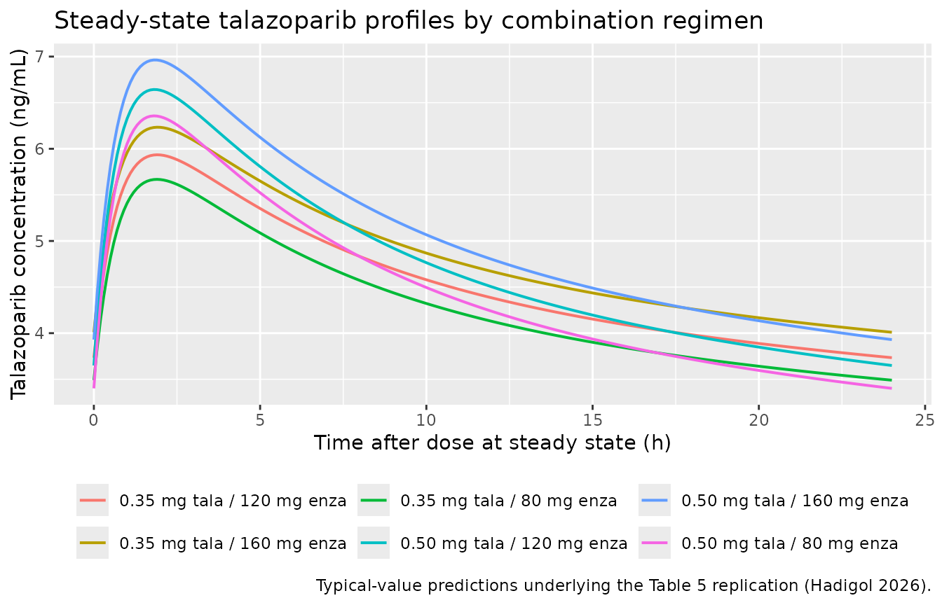

Perpetrator exposure and the time course of inhibition

The interaction is driven by Ce + Cn, which the paper never tabulates. Both species are long-lived relative to the 24 h dosing interval (enzalutamide terminal half-life about 5 days, the metabolite about 8 to 10 days), so their concentrations are nearly flat across the interval and talazoparib clearance is almost – but not exactly – constant.

perp <- ref_solve |>
  dplyr::summarise(
    `Mean Cc_enz (ng/mL)` = mean(.data$Cc_enz),
    `Mean Cc_ndmenz (ng/mL)` = mean(.data$Cc_ndmenz),
    `Mean Ce + Cn (ng/mL)` = mean(.data$Cc_enz + .data$Cc_ndmenz),
    `Mean CL inhibition factor` = mean(.data$cl) / .data$cl0[1],
    `Peak-to-trough range of Ce + Cn (%)` =
      100 * (max(.data$Cc_enz + .data$Cc_ndmenz) / min(.data$Cc_enz + .data$Cc_ndmenz) - 1)
  )

# Independent sanity check on the perpetrator scale. Dose / (CL * tau) gives
# the average steady-state concentration in closed form, including the fixed
# Fmet for the metabolite. These are algebraic identities for a linear system,
# so a few percent tolerance covers only the within-interval curvature.
ce_closed <- 1000 * 160 / (0.425 * tau)
cn_closed <- 1000 * 0.634 * 160 / (0.286 * tau)
stopifnot(
  abs(perp$`Mean Cc_enz (ng/mL)` / ce_closed - 1) < 0.05,
  abs(perp$`Mean Cc_ndmenz (ng/mL)` / cn_closed - 1) < 0.05
)

# The linear inhibition form is not bounded below, so a large enough
# perpetrator exposure would drive the factor negative. At the typical
# regimen it must sit comfortably inside (0, 1).
stopifnot(perp$`Mean CL inhibition factor` > 0.5,
          perp$`Mean CL inhibition factor` < 1)

perp |>
  tidyr::pivot_longer(dplyr::everything(), names_to = "Quantity", values_to = "Value") |>
  knitr::kable(digits = 3,
               caption = "Perpetrator exposure at enzalutamide 160 mg QD steady state and the resulting talazoparib clearance inhibition (typical values).")

Perpetrator exposure at enzalutamide 160 mg QD steady state and the resulting talazoparib clearance inhibition (typical values).
Quantity	Value
Mean Cc_enz (ng/mL)	15680.599
Mean Cc_ndmenz (ng/mL)	14777.656
Mean Ce + Cn (ng/mL)	30458.255
Mean CL inhibition factor	0.800
Peak-to-trough range of Ce + Cn (%)	13.982

ref_solve |>
  dplyr::select(tad, Enzalutamide = Cc_enz, `N-desmethyl enzalutamide` = Cc_ndmenz) |>
  tidyr::pivot_longer(-tad, names_to = "Analyte", values_to = "Conc") |>
  ggplot(aes(.data$tad, .data$Conc, colour = .data$Analyte)) +
  geom_line(linewidth = 0.7) +
  expand_limits(y = 0) +
  labs(x = "Time after dose at steady state (h)", y = "Concentration (ng/mL)",
       colour = NULL,
       title = "Perpetrator concentrations over one steady-state interval",
       caption = "Enzalutamide 160 mg QD; typical values (Hadigol 2026).") +
  theme(legend.position = "bottom")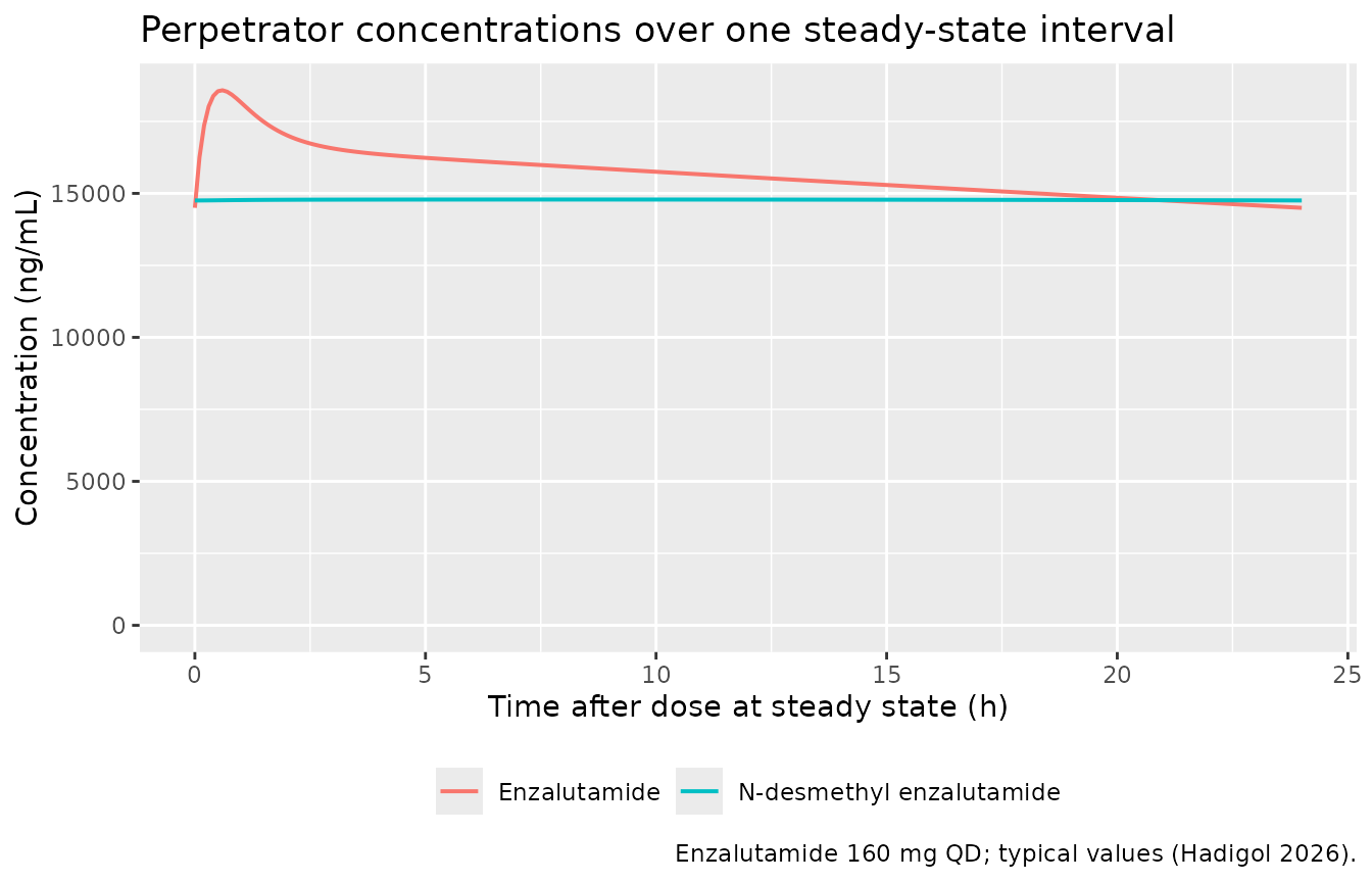

Virtual cohort

Original observed data are not publicly available, and the demographics table is not open access, so the cohort below uses covariate distributions consistent with the medians the main text names and with the renal-function strata the paper simulates. It exists to exercise the three variability blocks and to show the spread of the interaction across subjects – not to reproduce a published VPC, since Figure 3’s underlying data are not available.

# set.seed() seeds R's RNG, which is what draws the covariates below. It does
# NOT seed rxode2's simulation RNG, and rxode2 partitions its streams per
# solver thread, so the eta draws differ on a machine with a different thread
# count. Every assertion below is therefore written to hold for any cohort the
# model can produce (pattern 12 of the known-failure catalogue).
set.seed(20260912)

n_per_arm <- 100L   # cap is 200 per arm; 100 is ample here
n_day_cohort <- 84L # 12 weeks, past steady state for all three analytes

make_arm <- function(n, enza_dose, label, id_offset) {
  subj <- tibble::tibble(
    id = id_offset + seq_len(n),
    WT = pmin(150, pmax(45, rnorm(n, 80.1, 14))),
    AGE = pmin(92, pmax(40, rnorm(n, 71, 8))),
    CRCL = pmin(160, pmax(20, rnorm(n, 86.85, 25))),
    treatment = label
  )
  t_ss <- (n_day_cohort - 1L) * tau
  obs_t <- sort(unique(c(seq(0, t_ss, by = tau), seq(t_ss, t_ss + tau, by = 1))))
  doses <- subj |>
    tidyr::expand_grid(tibble::tibble(
      amt = c(0.5, enza_dose), cmt = c("depot", "depot_enz")
    )) |>
    dplyr::mutate(time = 0, evid = 1L, dvid = NA_integer_,
                  ii = tau, addl = n_day_cohort - 1L)
  obs <- subj |>
    tidyr::expand_grid(tibble::tibble(time = obs_t)) |>
    dplyr::mutate(amt = NA_real_, evid = 0L, cmt = "central", dvid = 1L,
                  ii = 0, addl = 0L)
  dplyr::bind_rows(doses, obs) |> dplyr::arrange(.data$id, .data$time, dplyr::desc(.data$evid))
}

events <- dplyr::bind_rows(
  make_arm(n_per_arm, 160, "160 mg enzalutamide", id_offset = 0L),
  make_arm(n_per_arm,  80,  "80 mg enzalutamide", id_offset = n_per_arm)
)

stopifnot(!anyDuplicated(unique(events[, c("id", "time", "evid")])))

sim <- rxode2::rxSolve(
  mod, events,
  useLinCmt = FALSE,
  keep = c("treatment", "WT", "AGE", "CRCL"),
  returnType = "data.frame"
)

stopifnot(nrow(sim) > 0, !anyNA(sim$Cc), all(sim$Cc >= 0))

# The linear inhibition term has no lower bound by construction, so confirm
# that no simulated subject is driven to a non-positive clearance. This is a
# structural guard on the extrapolation range, not a published number.
stopifnot(all(sim$cl > 0), all(sim$cl / sim$cl0 <= 1))

t_ss_c <- (n_day_cohort - 1L) * tau

sim |>
  dplyr::filter(.data$time >= t_ss_c) |>
  dplyr::mutate(tad = .data$time - t_ss_c) |>
  dplyr::group_by(.data$treatment, .data$tad) |>
  dplyr::summarise(
    Q05 = quantile(.data$Cc, 0.05), Q50 = median(.data$Cc),
    Q95 = quantile(.data$Cc, 0.95), .groups = "drop"
  ) |>
  ggplot(aes(.data$tad, .data$Q50)) +
  geom_ribbon(aes(ymin = .data$Q05, ymax = .data$Q95), alpha = 0.25) +
  geom_line(linewidth = 0.7) +
  facet_wrap(~treatment) +
  labs(x = "Time after dose at steady state (h)",
       y = "Talazoparib concentration (ng/mL)",
       title = "Simulated steady-state talazoparib exposure, median and 5th-95th percentile",
       caption = "Talazoparib 0.5 mg QD; 100 subjects per enzalutamide arm (Hadigol 2026 model).")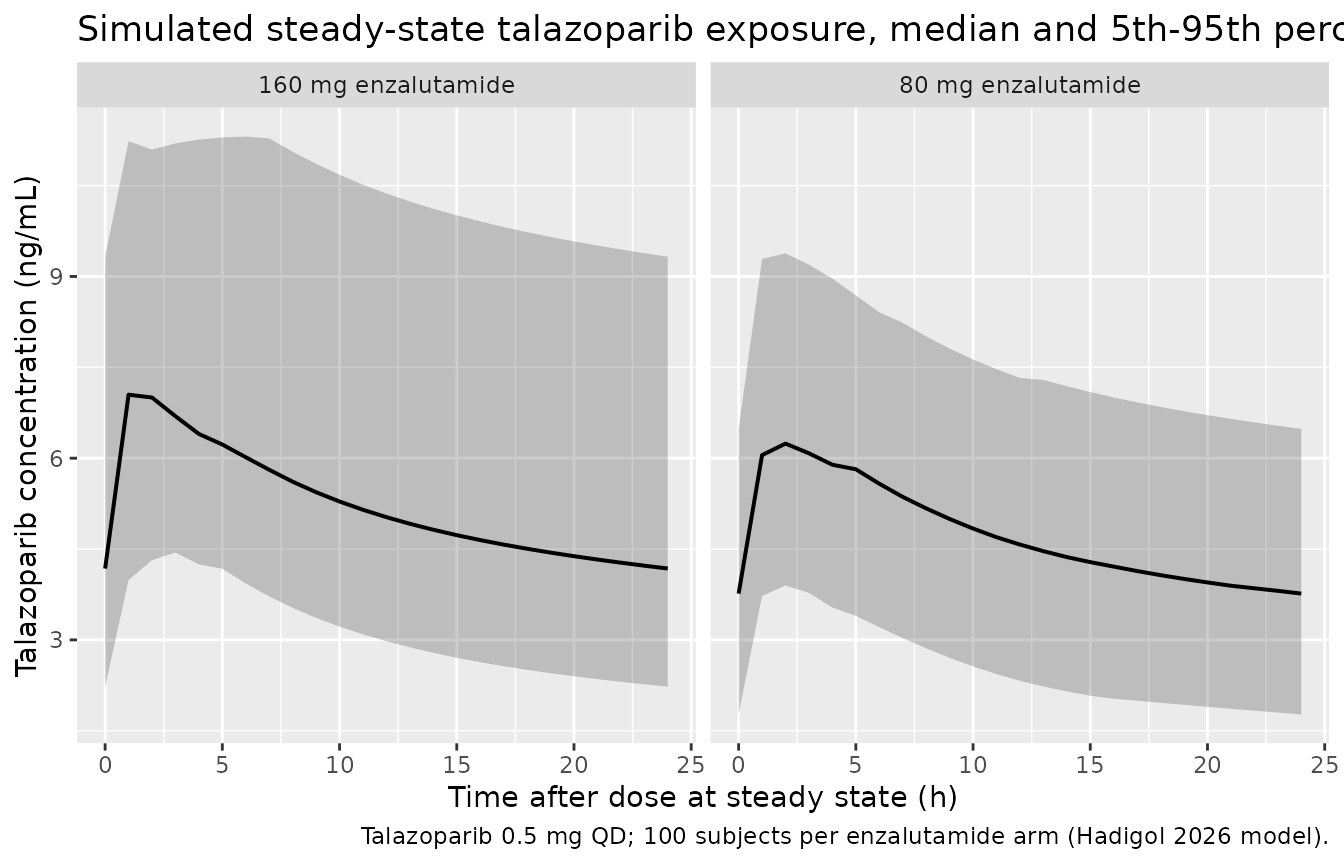

inhib <- sim |>
  dplyr::filter(.data$time >= t_ss_c) |>
  dplyr::group_by(.data$treatment, .data$id) |>
  dplyr::summarise(factor = mean(.data$cl) / dplyr::first(.data$cl0), .groups = "drop") |>
  dplyr::group_by(.data$treatment) |>
  dplyr::summarise(
    `Median CL inhibition factor` = median(.data$factor),
    `5th percentile` = quantile(.data$factor, 0.05),
    `95th percentile` = quantile(.data$factor, 0.95),
    .groups = "drop"
  )

# Cohort-derived, so bounds are on magnitude with generous headroom rather
# than on ordering or on one observed run. The 160 mg arm must show more
# inhibition than the 80 mg arm as an ABSOLUTE statement (the typical-value
# factors are ~0.80 and ~0.90, a 10-point separation that no plausible cohort
# draw closes), and neither arm may leave (0, 1).
stopifnot(
  all(inhib$`Median CL inhibition factor` > 0.5),
  all(inhib$`Median CL inhibition factor` < 1),
  inhib$`Median CL inhibition factor`[inhib$treatment == "160 mg enzalutamide"] < 0.87,
  inhib$`Median CL inhibition factor`[inhib$treatment == "80 mg enzalutamide"] > 0.84
)

inhib |>
  dplyr::rename("Enzalutamide arm" = treatment) |>
  knitr::kable(digits = 3,
               caption = "Distribution of the talazoparib clearance inhibition factor across the simulated cohort.")

Distribution of the talazoparib clearance inhibition factor across the simulated cohort.
Enzalutamide arm	Median CL inhibition factor	5th percentile	95th percentile
160 mg enzalutamide	0.791	0.731	0.845
80 mg enzalutamide	0.900	0.866	0.926

PKNCA on the cohort, all three analytes

One PKNCA block per output, each with its own concentration object, over the final steady-state dosing interval. The metabolite has no dose record of its own, so its PKNCA dose object carries the enzalutamide dose that ultimately generates it; only interval-bounded parameters (Cmax, Cmin, AUC over the interval, Cav) are requested, none of which depends on the dose amount.

enza_by_arm <- c("160 mg enzalutamide" = 160, "80 mg enzalutamide" = 80)

nca_one <- function(conc_col, dose_amt_fn) {
  cdat <- sim |>
    dplyr::filter(.data$time >= t_ss_c) |>
    dplyr::mutate(tad = .data$time - t_ss_c, Cc = .data[[conc_col]]) |>
    dplyr::filter(!is.na(.data$Cc)) |>
    dplyr::select(id, treatment, time = tad, Cc)
  stopifnot(nrow(cdat) > 0)

  ddat <- cdat |>
    dplyr::distinct(.data$id, .data$treatment) |>
    dplyr::mutate(time = 0, amt = dose_amt_fn(.data$treatment))

  co <- PKNCA::PKNCAconc(as.data.frame(cdat), Cc ~ time | treatment + id,
                         concu = "ng/mL", timeu = "h")
  do <- PKNCA::PKNCAdose(as.data.frame(ddat), amt ~ time | treatment + id,
                         route = "extravascular", doseu = "mg")
  PKNCA::pk.nca(PKNCA::PKNCAdata(co, do, intervals = data.frame(
    start = 0, end = tau, cmax = TRUE, cmin = TRUE, tmax = TRUE,
    auclast = TRUE, cav = TRUE
  )))
}

nca_tala   <- nca_one("Cc",        function(tr) 0.5)
nca_enz    <- nca_one("Cc_enz",    function(tr) unname(enza_by_arm[as.character(tr)]))
nca_ndmenz <- nca_one("Cc_ndmenz", function(tr) unname(enza_by_arm[as.character(tr)]))

summarise_nca <- function(res, analyte) {
  as.data.frame(res$result) |>
    dplyr::filter(.data$PPTESTCD %in% c("cmax", "cmin", "tmax", "auclast", "cav")) |>
    dplyr::group_by(.data$treatment, .data$PPTESTCD) |>
    dplyr::summarise(median = median(.data$PPORRES), .groups = "drop") |>
    tidyr::pivot_wider(names_from = "PPTESTCD", values_from = "median") |>
    dplyr::mutate(Analyte = analyte, .before = 1)
}

nca_all <- dplyr::bind_rows(
  summarise_nca(nca_tala, "Talazoparib"),
  summarise_nca(nca_enz, "Enzalutamide"),
  summarise_nca(nca_ndmenz, "N-desmethyl enzalutamide")
)

stopifnot(nrow(nca_all) == 6L, !anyNA(nca_all$auclast))

nca_all |>
  dplyr::rename(
    "Arm" = treatment,
    "Cmax,ss (ng/mL)" = cmax,
    "Cmin,ss (ng/mL)" = cmin,
    "Tmax (h)" = tmax,
    "AUC0-24,ss (ng*h/mL)" = auclast,
    "Cav,ss (ng/mL)" = cav
  ) |>
  knitr::kable(digits = 2,
               caption = "Cohort-median steady-state NCA for all three analytes, by enzalutamide arm (PKNCA).")

Cohort-median steady-state NCA for all three analytes, by enzalutamide arm (PKNCA).
Analyte	Arm	AUC0-24,ss (ng*h/mL)	Cav,ss (ng/mL)	Cmax,ss (ng/mL)	Cmin,ss (ng/mL)	Tmax (h)
Talazoparib	160 mg enzalutamide	127.22	5.30	7.32	4.18	2.0
Talazoparib	80 mg enzalutamide	116.21	4.84	6.43	3.76	2.0
Enzalutamide	160 mg enzalutamide	383259.32	15969.14	18643.54	15121.22	1.0
Enzalutamide	80 mg enzalutamide	186874.75	7786.45	8920.91	7186.65	1.0
N-desmethyl enzalutamide	160 mg enzalutamide	354123.66	14755.15	14769.98	14718.03	8.5
N-desmethyl enzalutamide	80 mg enzalutamide	173983.20	7249.30	7255.74	7232.56	9.0

Two qualitative cross-checks against published pharmacology, neither of which Hadigol 2026 tabulates and so neither of which is a gate:

enz_cav <- nca_all$cav[nca_all$Analyte == "Enzalutamide" &
                         nca_all$treatment == "160 mg enzalutamide"]
ndm_cav <- nca_all$cav[nca_all$Analyte == "N-desmethyl enzalutamide" &
                         nca_all$treatment == "160 mg enzalutamide"]

# Enzalutamide and its N-desmethyl metabolite circulate at broadly comparable
# steady-state concentrations at 160 mg QD, which is why the paper treats their
# summed concentration as the perpetrator driver. Magnitude bound only.
stopifnot(ndm_cav / enz_cav > 0.4, ndm_cav / enz_cav < 2.5)

tibble::tribble(
  ~Quantity, ~Model, ~`Published expectation`,
  "Enzalutamide Cav,ss at 160 mg QD (ng/mL)", sprintf("%.0f", enz_cav),
  "about 10,000-16,000 (label range; not tabulated in Hadigol 2026)",
  "N-desmethyl / enzalutamide Cav,ss ratio", sprintf("%.2f", ndm_cav / enz_cav),
  "near 1; the two are comparable and equipotent (Methods)"
) |>
  knitr::kable(caption = "Qualitative cross-checks against published enzalutamide pharmacology. Not gated.")

Qualitative cross-checks against published enzalutamide pharmacology. Not gated.
Quantity	Model	Published expectation
Enzalutamide Cav,ss at 160 mg QD (ng/mL)	15969	about 10,000-16,000 (label range; not tabulated in Hadigol 2026)
N-desmethyl / enzalutamide Cav,ss ratio	0.92	near 1; the two are comparable and equipotent (Methods)

Assumptions and deviations

Covariate distributions are assumed. Hadigol 2026 Tables S1 and S2 (study population summary and baseline demographics) are not open access. The virtual cohort therefore draws body weight, age and baseline creatinine clearance from normal distributions centred on the medians the main text names (80.1 kg, 71 years) and on the 86.85 mL/min reference, truncated to physiologically plausible ranges. No published covariate range, race/ethnicity split or regional split could be recorded in the model’s population metadata. The cohort figures are illustrative; they are not a reproduction of the paper’s Figure 3 pvcVPC, whose underlying observations are not available.
86.85 mL/min is not claimed to be a median. The paper introduces it only as the baseline creatinine clearance of the typical patient in equation (6). With the demographics table unavailable there is no way to confirm it is the cohort median, so neither the model file nor this vignette describes it as one. By contrast 80.1 kg and 71 years are explicitly stated as population medians (Table 5 Note).
The creatinine-clearance assay is not named. Hadigol 2026 never states which equation produced BCCL. The raw-mL/min renal-disease cutoffs of its Table 4 (normal > 90, mild 60-89, moderate 30-59, severe 15-29) are the only evidence for the normalisation, and they imply a raw, non-BSA-normalised clearance. The model’s covariateData[[CRCL]] records this explicitly, because supplying a BSA-normalised value instead would silently rescale the renal effect.
Residual error is encoded as log-normal, matching “additive on log-transformed data”. All three tables report a “Thetarized sigma” – the NONMEM idiom in which $SIGMA is fixed to 1 and the residual SD is carried as an estimated THETA – and the Results state the talazoparib value is “the additive residual variability for log-transformed observation data”. nlmixr2 expresses that exactly as lnorm(expSd), so the printed SDs are used directly with no CV conversion.
No molar-mass correction on metabolite formation. Hadigol 2026 gives Fmet = 0.634 with no statement about whether it is a mass or molar fraction, and the metabolite differs from the parent by one methyl group (about 3% of the molecular mass). The model routes fm times the enzalutamide mass flux into the metabolite compartment, i.e. treats it as a mass fraction, which is what reproduces the paper’s own numbers. Since Fmet was fixed rather than estimated and is confounded with Vcn, a molar reinterpretation would be absorbed into Vcn and would not change predicted concentrations.
The interaction term is linear and therefore unbounded below. Equation (1) has no Imax; the factor (1 - 6.58e-6 * (Ce + Cn)) reaches zero at a combined perpetrator concentration of about 152,000 ng/mL, roughly five times the typical steady-state value at 160 mg QD. That is far outside the observed range and the simulated cohort stays well clear of it (minimum factor about 0.65), but the model asserts cl > 0 across the cohort rather than assuming it, and the form should not be extrapolated to enzalutamide exposures far above the therapeutic range.
The body-weight exponent on enzalutamide Vce/Fe is 3.495. This is far above any allometric value and makes the central volume very sensitive to weight (about 9 L at 60 kg versus about 55 L at 100 kg). It is transcribed as printed: Table 1 reports it with SE 0.279, RSE 7.99% and a SIR 95% CI of [3.105, 3.904], all of which confirm the magnitude, and the paper notes these covariates are not clinically significant and warrant no dose adjustment.
Covariates screened but not retained are recorded, not encoded. Moderate CYP3A4 inhibitors (on both CLe/Fe and CLn), moderate P-gp inhibitors (on Ft and kat), race (Asian versus non-Asian) and region (Chinese versus non-Chinese) were all tested and rejected, and no point estimate is published for any of them. They appear in the model’s covariatesDataExcluded metadata so the provenance of the covariate screen survives, without carrying convention warnings for declared-but-unused covariates.
Absorption is sparsely informed. Dense sampling was designed only for Part 1 (19 of 811 patients); Part 2 used sparse sampling. Food status, a covariate on talazoparib kat in the monotherapy model, was not available for the combination and the paper flags this as a limitation. Only the hard-capsule formulation was used, so the monotherapy model’s formulation effect on kat does not appear here either.
Base models and the sequential-fit intermediates are not extracted. Tables S4 to S8 (base models for each analyte and the model-selection summaries) are not open access, and in any case only the final model of each sequential stage is a published result. The packaged model carries the three final models as one coupled system, which is how the paper uses them.
No cross-analyte random-effect covariance. The three sub-models were fit sequentially with upstream parameters fixed to empirical Bayes estimates, so no such covariance was estimated and none is invented. The model has three independent variability blocks: a 2x2 block for enzalutamide, a 2x2 block for the metabolite, and two diagonal etas for talazoparib.
All parameter values come from the paper’s main-text tables and numbered equations. No value was digitised from a figure, obtained by correspondence, or carried from an upstream model file.