Model and source
mod <- readModelDb("Lin_2021_vancomycin")
mod_ui <- rxode2::rxode2(mod)
#> ℹ parameter labels from comments will be replaced by 'label()'
mod_meta <- mod_ui$meta- Citation: Lin Z, Chen DY, Zhu YW, Jiang ZL, Cui K, Zhang S, Chen LH. Population pharmacokinetic modeling and clinical application of vancomycin in Chinese patients hospitalized in intensive care units. Sci Rep. 2021;11(1):2670. doi:10.1038/s41598-021-82312-2
- Description: One-compartment IV population PK model for vancomycin in adult Chinese ICU patients, with additive-linear covariate equations on CL (dopamine co-medication, serum creatinine, severe-burn status, total body weight, CRRT status) and on V (serum creatinine, age, total body weight) and additive-normal between-subject variability, fitted by the EM algorithm in Kinetica (Lin 2021)
- Article (DOI): https://doi.org/10.1038/s41598-021-82312-2
Lin 2021 fitted a one-compartment model to sparse steady-state vancomycin troughs and “approach peak” concentrations from adult ICU patients at Taizhou Hospital (Zhejiang, China), using the expectation-maximisation (EM) algorithm in Kinetica 4.4.1. Covariates enter as additive-linear equations with no centring (Tables 3 and 4):
CL (L/h) = 0.78 + 0.036*DA - 0.007*Cr - 0.43*Burn-S + 0.067*TBW + 0.41*CRRT-S
V  (L)   = 46.47 - 0.04*Cr - 0.07*Age + 0.16*TBW
where DA, Burn-S and CRRT-S are coded 1 or 2 (Methods): DA 1 = no
dopamine, 2 = dopamine; Burn-S 1 = burn degree > 50% in acute
convalescence, 2 = otherwise; CRRT-S 1 = treated by CRRT, 2 = not. The
packaged model takes the canonical 0/1 indicators
CONMED_DOPA, DIS_BURN_RECENT and
RRT_CRRT_STATUS and rebuilds the source codes inside
model(), so the printed coefficients are used unchanged.
Between-subject variability is additive-normal on the linear parameters
(Methods: beta_i = Z_i beta + eta_j).
Population
The study enrolled 466 adult ICU patients between July 2015 and December 2017: 294 for model building, 80 for external validation (374 in total, summarised in Table 1) and 92 for a Bayesian dose-adjustment application. Of the 374, 254 (67.9%) were male. Median age was 62 years (range 18-93), median total body weight 65.0 kg (40.0-90.6) and median serum creatinine 71.0 umol/L (28.0-581.0). 87 (23.3%) were on continuous renal replacement therapy and 32 (8.6%) had burns. Infection sites were blood 55.6%, pulmonary 18.2%, skin and soft tissue 11.2%, abdominal 6.4% and other 8.6%. Regimens were 0.5 g qd, q12h, q8h or q6h, or 1 g qd or q12h, chosen by the clinicians. There were 837 troughs (0.5 h before the next dose) and 156 approach-peak samples (1 h after the end of infusion), mostly after the 6th dose. Observed means were 16.3 +/- 12.4 ug/mL (trough) and 36.0 +/- 19.4 ug/mL (approach peak).
Source trace
| Element | Value | Source |
|---|---|---|
| Structure | one compartment, IV infusion, first-order elimination | Methods (‘we fit the data with a one-compartment model’) |
CL intercept lcl_int
|
0.78 L/h | Table 6 theta1; Table 3 final equation |
DA slope e_conmed_dopa_cl
|
+0.036 L/h per code unit | Table 6 theta2; Table 3 |
Cr slope on CL e_creat_cl
|
-0.007 L/h per umol/L | Table 6 theta3; Table 3 |
Burn-S slope e_dis_burn_recent_cl
|
-0.43 L/h per code unit | Table 6 theta4; Table 3 |
TBW slope on CL e_wt_cl
|
+0.067 L/h per kg | Table 6 theta5; Table 3 |
CRRT-S slope e_rrt_crrt_status_cl
|
+0.41 L/h per code unit | Table 6 theta6; Table 3 |
V intercept lvc_int
|
46.47 L | Table 6 theta7; Table 4 final equation |
Cr slope on V e_creat_vc
|
-0.04 L per umol/L | Table 6 theta8; Table 4 |
Age slope on V e_age_vc
|
-0.07 L per year | Table 6 theta9; Table 4 |
TBW slope on V e_wt_vc
|
+0.16 L per kg | Table 6 theta10; Table 4 |
etacl variance |
(0.4172 x 3.16)^2 = 1.7381 (L/h)^2 | Table 6 final ‘%CV of CL’ 41.72% and population CL 3.16 L/h |
etavc variance |
(0.3514 x 60.71)^2 = 455.11 L^2 | Table 6 final ‘%CV of V’ 35.14% and population V 60.71 L |
| Covariate codes (DA, Burn-S, CRRT-S) | 1 / 2 | Methods, covariate list; Table 1 |
Residual error addSd
|
fixed 0 (not reported) | – |
Table 6 prints the magnitudes of theta3, theta4, theta8 and theta9 without signs; the signs come from the printed equations (Tables 3, 4 and 7 and the Results text, which all agree). Every sign matches the direction stated in the abstract and Discussion, which the deterministic checks below confirm.
Deterministic checks of the covariate equations
The typical values are solved with the random effects set to zero and compared with the printed equations evaluated by hand.
eq_cl <- function(dopa, creat, burn, wt, crrt) {
  0.78 + 0.036 * (dopa + 1) - 0.007 * creat - 0.43 * (2 - burn) +
    0.067 * wt + 0.41 * (2 - crrt)
}
eq_vc <- function(creat, age, wt) 46.47 - 0.04 * creat - 0.07 * age + 0.16 * wt

grid <- expand.grid(
  CONMED_DOPA = 0:1, DIS_BURN_RECENT = 0:1, RRT_CRRT_STATUS = 0:1,
  CREAT = c(40, 71, 200), WT = c(50, 65, 85), AGE = c(30, 62, 85)
)
grid$id <- seq_len(nrow(grid))
ev_grid <- grid |>
  dplyr::mutate(time = 0, evid = 0, cmt = "central", amt = 0)

mod0 <- rxode2::zeroRe(mod)
#> ℹ parameter labels from comments will be replaced by 'label()'
# zeroRe() warns that a multi-subject solve has no omega; the etas are either
# zero (typical values) or supplied as data columns, so that is intended.
solve0 <- function(events, ...) {
  withCallingHandlers(
    suppressMessages(rxode2::rxSolve(mod0, events = events, returnType = "data.frame", ...)),
    warning = function(w) {
      if (grepl("omega", conditionMessage(w))) invokeRestart("muffleWarning")
    }
  )
}
tv <- solve0(ev_grid) |>
  dplyr::select(id, tvcl, tvvc) |>
  dplyr::left_join(grid, by = "id") |>
  dplyr::mutate(
    cl_eq = eq_cl(CONMED_DOPA, CREAT, DIS_BURN_RECENT, WT, RRT_CRRT_STATUS),
    vc_eq = eq_vc(CREAT, AGE, WT)
  )
stopifnot(
  nrow(tv) == nrow(grid),
  max(abs(tv$tvcl - tv$cl_eq)) < 1e-10,
  max(abs(tv$tvvc - tv$vc_eq)) < 1e-10
)

# Effect of each binary indicator, holding everything else fixed. These are
# exact differences, and their signs are the directions the paper states.
eff <- function(var) {
  base <- tv[tv[[var]] == 0, ]
  alt <- tv[tv[[var]] == 1, ]
  key <- setdiff(names(grid), c(var, "id"))
  m <- merge(base, alt, by = key, suffixes = c(".0", ".1"))
  stopifnot(nrow(m) == nrow(grid) / 2)
  unique(round(m$tvcl.1 - m$tvcl.0, 10))
}
d_dopa <- eff("CONMED_DOPA")
d_burn <- eff("DIS_BURN_RECENT")
d_crrt <- eff("RRT_CRRT_STATUS")
stopifnot(
  length(d_dopa) == 1, abs(d_dopa - 0.036) < 1e-9, # dopamine raises CL
  length(d_burn) == 1, abs(d_burn - 0.43) < 1e-9, # severe burn raises CL
  length(d_crrt) == 1, abs(d_crrt + 0.41) < 1e-9 # CRRT lowers CL
)

knitr::kable(
  data.frame(
    Indicator = c("Dopamine (CONMED_DOPA = 1)", "Severe acute burn (DIS_BURN_RECENT = 1)", "CRRT (RRT_CRRT_STATUS = 1)"),
    `Change in CL (L/h)` = c(d_dopa, d_burn, d_crrt),
    `Paper statement` = c("CL raised with dopamine", "CL raised with severe burn", "CL reduced with CRRT"),
    check.names = FALSE
  ),
  caption = "Change in typical CL for each binary covariate (all other covariates held fixed)."
)| Indicator | Change in CL (L/h) | Paper statement |
|---|---|---|
| Dopamine (CONMED_DOPA = 1) | 0.036 | CL raised with dopamine |
| Severe acute burn (DIS_BURN_RECENT = 1) | 0.430 | CL raised with severe burn |
| CRRT (RRT_CRRT_STATUS = 1) | -0.410 | CL reduced with CRRT |
Typical values at the cohort medians versus the printed population values
The Results and abstract report population values of CL = 3.16 L/h and V = 60.71 L for the final model. The printed equations evaluated at the Table 1 medians do not return those numbers:
ref <- data.frame(
  id = 1L, time = 0, evid = 0, cmt = "central", amt = 0,
  CONMED_DOPA = 0, DIS_BURN_RECENT = 0, RRT_CRRT_STATUS = 0,
  CREAT = 71, WT = 65, AGE = 62
)
ref_tv <- solve0(ref)
stopifnot(
  abs(ref_tv$tvcl - 4.6341) < 1e-4,
  abs(ref_tv$tvvc - 49.69) < 1e-4
)
knitr::kable(
  data.frame(
    Parameter = c("CL (L/h)", "V (L)"),
    `Equation at Table 1 medians` = signif(c(ref_tv$tvcl, ref_tv$tvvc), 4),
    `Printed population value` = c(3.16, 60.71),
    Ratio = signif(c(ref_tv$tvcl / 3.16, ref_tv$tvvc / 60.71), 3),
    check.names = FALSE
  ),
  caption = "Reference subject: no dopamine, no burn, no CRRT, Cr 71 umol/L, TBW 65 kg, age 62 years."
)| Parameter | Equation at Table 1 medians | Printed population value | Ratio |
|---|---|---|---|
| CL (L/h) | 4.634 | 3.16 | 1.470 |
| V (L) | 49.690 | 60.71 | 0.818 |
The gap cannot come from the choice of reference subject. The equations are linear, so the mean of the typical values equals the equation evaluated at the mean covariates. A creatinine mean above the median lowers CL, but reaching 3.16 L/h at otherwise median covariates needs a mean creatinine of about 280 umol/L (the median is 71). No plausible covariate mean raises V from 49.7 L to 60.71 L: even with creatinine and age at their Table 1 minima (28 umol/L, 18 years), TBW would have to be about 104 kg, above the cohort maximum of 90.6 kg. The paper therefore reports the population values and the covariate equations inconsistently. The packaged model encodes the printed equations, since those are what a user applies to a patient. The printed 3.16 L/h and 60.71 L are used only to convert the reported %CV into eta standard deviations. The same value, V = 60.71 L, also appears for the unrelated Yasuhara model in the paper’s Table 7.
Where the CL equation crosses zero
Because the CL equation is additive-linear, it becomes negative at a high creatinine combined with a low weight:
zc <- expand.grid(WT = c(40, 50, 65, 90.6), RRT_CRRT_STATUS = 0:1) |>
  dplyr::mutate(
    `Cr at which typical CL = 0 (umol/L)` =
      round((eq_cl(0, 0, 0, WT, RRT_CRRT_STATUS)) / 0.007)
  ) |>
  dplyr::rename(`TBW (kg)` = WT, CRRT = RRT_CRRT_STATUS)
stopifnot(all(zc$`Cr at which typical CL = 0 (umol/L)` > 400))
knitr::kable(zc, caption = "Creatinine at which the typical CL reaches zero (no dopamine, no burn).")| TBW (kg) | CRRT | Cr at which typical CL = 0 (umol/L) |
|---|---|---|
| 40.0 | 0 | 494 |
| 50.0 | 0 | 589 |
| 65.0 | 0 | 733 |
| 90.6 | 0 | 978 |
| 40.0 | 1 | 435 |
| 50.0 | 1 | 531 |
| 65.0 | 1 | 674 |
| 90.6 | 1 | 919 |
Every zero-crossing lies above 400 umol/L. It falls inside the observed creatinine range (up to 581 umol/L) only for patients weighing about 50 kg or less. Do not use the model for patients with both a high creatinine and a low weight: its typical CL there is close to zero or negative.
Virtual cohort
The cohort follows the Table 1 marginals. Correlations between
covariates are not reported, so covariates are drawn independently.
Draws are rejected and redrawn, never clamped, to stay inside the
observed ranges. The etas are drawn in base R, and the solve uses
zeroRe() with the etas supplied as data columns. This keeps
the cohort identical on every machine.
set.seed(20210129)
n_per_arm <- 200
arms <- data.frame(
  treatment = c("0.5 g q12h", "1 g q12h"),
  amt = c(500, 1000),
  ii = c(12, 12)
)

draw_trunc <- function(n, rfun, lo, hi) {
  out <- numeric(0)
  while (length(out) < n) {
    x <- rfun(n)
    out <- c(out, x[x >= lo & x <= hi])
  }
  out[seq_len(n)]
}

make_cohort <- function(n) {
  data.frame(
    AGE = draw_trunc(n, function(k) rnorm(k, 62, 16), 18, 93),
    WT = draw_trunc(n, function(k) rnorm(k, 65, 10), 40, 90.6),
    CREAT = draw_trunc(n, function(k) rlnorm(k, log(71), 0.6), 28, 581),
    RRT_CRRT_STATUS = rbinom(n, 1, 0.233),
    DIS_BURN_RECENT = rbinom(n, 1, 0.086),
    CONMED_DOPA = rbinom(n, 1, 0.2),
    etacl = rnorm(n, 0, sqrt(1.7381)),
    etavc = rnorm(n, 0, sqrt(455.11))
  )
}

cohort <- dplyr::bind_rows(lapply(seq_len(nrow(arms)), function(i) {
  cbind(make_cohort(n_per_arm), treatment = arms$treatment[i], amt = arms$amt[i], ii = arms$ii[i])
}))
cohort$id <- seq_len(nrow(cohort))
cohort <- cohort |>
  dplyr::mutate(
    cl_i = eq_cl(CONMED_DOPA, CREAT, DIS_BURN_RECENT, WT, RRT_CRRT_STATUS) + etacl,
    vc_i = eq_vc(CREAT, AGE, WT) + etavc
  )
n_nonpos <- sum(cohort$cl_i <= 0 | cohort$vc_i <= 0)
n_nonpos
#> [1] 5
With additive-normal etas a draw can give a non-positive CL or V. In
this cohort 5 of 400 subjects did, and they are removed before
simulation. The model has no guard against this; a user drawing from
omega should check cl > 0 and
vc > 0. The V eta SD (21.3 L) is large relative to the
typical V (about 50 L), so some retained subjects also have an
implausibly small V: 6 have V below 10 L.
Simulation
Each subject receives the arm’s dose at steady state
(ss = 1). The paper does not report the infusion duration;
1 h is assumed, which fits the approach-peak sample being defined as 1 h
after the end of infusion. The dosing interval is sampled densely.
t_inf <- 1
obs_times <- sort(unique(c(seq(0, 1.5, by = 0.05), seq(1.5, 12, by = 0.25))))

dose_rows <- cohort |>
  dplyr::transmute(
    id, time = 0, evid = 1, cmt = "central", amt, rate = amt / t_inf,
    ii, ss = 1, treatment, AGE, WT, CREAT, RRT_CRRT_STATUS,
    DIS_BURN_RECENT, CONMED_DOPA, etacl, etavc
  )
obs_rows <- cohort |>
  dplyr::select(id, treatment, AGE, WT, CREAT, RRT_CRRT_STATUS, DIS_BURN_RECENT, CONMED_DOPA, etacl, etavc) |>
  tidyr::crossing(time = obs_times) |>
  dplyr::mutate(evid = 0, cmt = "central", amt = 0, rate = 0, ii = 0, ss = 0)
ev <- dplyr::bind_rows(dose_rows, obs_rows) |>
  dplyr::arrange(id, time, dplyr::desc(evid))

sim <- solve0(
  ev,
  keep = "treatment",
  rtol = 1e-10, atol = 1e-12, ssRtol = 1e-10, ssAtol = 1e-12
)

# The model uses the data etas: individual CL matches the hand calculation.
chk_cl <- sim |>
  dplyr::distinct(id, cl, vc) |>
  dplyr::left_join(cohort |> dplyr::select(id, cl_i, vc_i), by = "id")
stopifnot(
  nrow(chk_cl) == nrow(cohort),
  max(abs(chk_cl$cl - chk_cl$cl_i)) < 1e-10,
  max(abs(chk_cl$vc - chk_cl$vc_i)) < 1e-10
)
Closed-form check at steady state
For a one-compartment infusion at steady state, the concentration at
the end of infusion is
(R/CL) (1 - exp(-k Tinf)) / (1 - exp(-k tau)), and the
concentration decays mono-exponentially from there. The ODE solve
reproduces this for every subject:
cf <- sim |>
  dplyr::left_join(cohort |> dplyr::select(id, amt), by = "id") |>
  dplyr::mutate(
    k = cl / vc,
    cend = (amt / t_inf / cl) * (1 - exp(-k * t_inf)) / (1 - exp(-k * 12)),
    ctrough = cend * exp(-k * (12 - t_inf)),
    closed = dplyr::if_else(
      time <= t_inf,
      ctrough * exp(-k * time) + (amt / t_inf / cl) * (1 - exp(-k * time)),
      cend * exp(-k * (time - t_inf))
    )
  )
# Error scaled by each subject's peak: subjects with a very small V (see
# below) decay to ~1e-60 ug/mL by the trough, where a ratio is meaningless.
rel_err <- cf |>
  dplyr::group_by(id) |>
  dplyr::summarise(e = max(abs(Cc - closed)) / max(closed)) |>
  dplyr::pull(e) |>
  max()
rel_err
#> [1] 1.710924e-09
stopifnot(rel_err < 1e-6)
Trough and approach-peak concentrations
tp <- sim |>
  dplyr::filter(time %in% c(2, 11.5)) |>
  dplyr::mutate(sample = ifelse(time == 2, "Approach peak (1 h after end of infusion)", "Trough (0.5 h before next dose)")) |>
  dplyr::group_by(treatment, sample) |>
  dplyr::summarise(
    n = dplyr::n(),
    `Median (ug/mL)` = signif(median(Cc), 3),
    `Mean (ug/mL)` = signif(mean(Cc), 3),
    `P5-P95 (ug/mL)` = paste(signif(quantile(Cc, 0.05), 3), signif(quantile(Cc, 0.95), 3), sep = " - "),
    .groups = "drop"
  )
stopifnot(nrow(tp) == 4, all(tp$n > 150))
tp_mean <- function(reg, smp) {
  v <- tp$`Mean (ug/mL)`[tp$treatment == reg & startsWith(tp$sample, smp)]
  if (length(v) != 1L) stop("no unique row for ", reg, " / ", smp)
  v
}
knitr::kable(tp, caption = "Simulated steady-state concentrations by regimen. Observed across all regimens (Table 1): trough 16.3 +/- 12.4, approach peak 36.0 +/- 19.4 ug/mL.")| treatment | sample | n | Median (ug/mL) | Mean (ug/mL) | P5-P95 (ug/mL) |
|---|---|---|---|---|---|
| 0.5 g q12h | Approach peak (1 h after end of infusion) | 198 | 14.60 | 16.50 | 9.52 - 26.5 |
| 0.5 g q12h | Trough (0.5 h before next dose) | 198 | 5.98 | 7.35 | 2.03 - 16.7 |
| 1 g q12h | Approach peak (1 h after end of infusion) | 197 | 28.20 | 34.30 | 18.8 - 53.9 |
| 1 g q12h | Trough (0.5 h before next dose) | 197 | 12.20 | 17.20 | 2.8 - 38.7 |
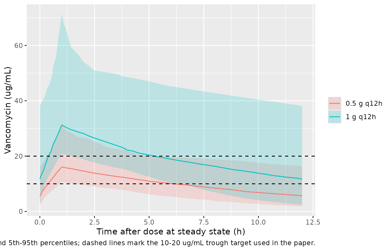
The paper does not give the regimen mix behind the Table 1 means, so these values are context rather than a gate. For 1 g q12h the simulated mean trough is 17.2 ug/mL and the mean approach peak 34.3 ug/mL, close to the observed 16.3 and 36.0 ug/mL. For 0.5 g q12h they are lower (7.35 and 16.5 ug/mL). Because the regimen mix is unknown, this comparison cannot decide between the equation typical values and the printed 3.16 L/h and 60.71 L discussed above.
sim |>
  dplyr::group_by(treatment, time) |>
  dplyr::summarise(
    p05 = quantile(Cc, 0.05), p50 = median(Cc), p95 = quantile(Cc, 0.95),
    .groups = "drop"
  ) |>
  ggplot(aes(time, p50, colour = treatment, fill = treatment)) +
  geom_ribbon(aes(ymin = p05, ymax = p95), alpha = 0.2, colour = NA) +
  geom_line() +
  geom_hline(yintercept = c(10, 20), linetype = "dashed") +
  labs(
    x = "Time after dose at steady state (h)", y = "Vancomycin (ug/mL)",
    colour = NULL, fill = NULL,
    caption = "Median and 5th-95th percentiles; dashed lines mark the 10-20 ug/mL trough target used in the paper."
  )
PKNCA validation
At steady state AUC(0-tau) = Dose / CL, whatever the
volume. The PKNCA interval AUC is checked against each subject’s own
clearance.
# Subjects with a very small V decay into integrator noise before the
# trough. Assert the undershoot is noise relative to each subject's peak,
# floor it at zero and drop the numerically-zero tail after the peak so the
# log-down trapezoid does not follow the noise.
conc <- sim |>
  dplyr::filter(!is.na(Cc)) |>
  dplyr::select(id, treatment, time, Cc) |>
  dplyr::group_by(id) |>
  dplyr::mutate(undershoot = min(Cc) / max(Cc)) |>
  dplyr::ungroup()
stopifnot(all(conc$undershoot > -1e-9))
conc <- conc |>
  dplyr::mutate(Cc = pmax(Cc, 0)) |>
  dplyr::group_by(id) |>
  dplyr::filter(time <= time[which.max(Cc)] | Cc >= 1e-9 * max(Cc)) |>
  dplyr::ungroup() |>
  dplyr::select(-undershoot)
dose_df <- cohort |>
  dplyr::transmute(id, treatment, time = 0, amt)

conc_obj <- PKNCA::PKNCAconc(conc, Cc ~ time | treatment + id)
dose_obj <- PKNCA::PKNCAdose(dose_df, amt ~ time | treatment + id)
intervals <- data.frame(
  start = 0, end = 12,
  auclast = TRUE, cmax = TRUE, tmax = TRUE, cmin = TRUE
)
nca <- PKNCA::pk.nca(PKNCA::PKNCAdata(conc_obj, dose_obj, intervals = intervals))
nca_df <- as.data.frame(nca$result)

auc_chk <- nca_df |>
  dplyr::filter(PPTESTCD == "auclast") |>
  dplyr::left_join(cohort |> dplyr::select(id, amt, cl_i), by = "id") |>
  dplyr::mutate(pct_diff = 100 * (PPORRES - amt / cl_i) / (amt / cl_i))
stopifnot(
  nrow(auc_chk) == nrow(cohort),
  max(abs(auc_chk$pct_diff)) < 0.5
)

nca_df |>
  dplyr::filter(PPTESTCD %in% c("auclast", "cmax", "cmin")) |>
  dplyr::group_by(treatment, PPTESTCD) |>
  dplyr::summarise(median = signif(median(PPORRES), 3), .groups = "drop") |>
  tidyr::pivot_wider(names_from = PPTESTCD, values_from = median) |>
  dplyr::rename(
    Regimen = treatment,
    `AUC0-12 (ug*h/mL)` = auclast,
    `Cmax (ug/mL)` = cmax,
    `Cmin (ug/mL)` = cmin
  ) |>
knitr::kable(caption = "Median steady-state NCA by regimen (simulated).")| Regimen | AUC0-12 (ug*h/mL) | Cmax (ug/mL) | Cmin (ug/mL) |
|---|---|---|---|
| 0.5 g q12h | 123 | 16.0 | 5.7 |
| 1 g q12h | 228 | 31.2 | 11.7 |
The paper reports no NCA summary, so no side-by-side NCA comparison is possible. The largest absolute difference between the PKNCA AUC(0-12) and Dose/CL across subjects was 0.3%.
Assumptions and deviations
- Covariate equations versus printed population values. The equations at the Table 1 medians give CL 4.63 L/h and V 49.7 L. The paper states population values of 3.16 L/h and 60.71 L. The model encodes the equations (see above).
- Coefficient signs. Table 6 lists theta3, theta4, theta8 and theta9 as magnitudes; the signs are taken from the equations printed in Tables 3, 4 and 7 and in the Results text. The CRRT coefficient lowers CL, as the abstract and Discussion state, even though the paper notes this contradicts earlier reports.
-
Covariate coding. The paper codes DA, Burn-S and
CRRT-S as 1/2. The model takes canonical 0/1 indicators
(
CONMED_DOPA = DA - 1,DIS_BURN_RECENT = 2 - Burn-S,RRT_CRRT_STATUS = 2 - CRRT-S) and rebuilds the codes internally. The Methods define Burn-S 2 as ‘burn degree < 50%, 20 days after burn’. Table 1 shows only ‘Burn’ versus ‘No burn’, so patients without burns are taken to carry code 2 as well. - Between-subject variability. Kinetica’s EM model adds normally distributed etas to the linear parameters. The eta SDs are the Table 6 %CV multiplied by the printed population values (3.16 L/h, 60.71 L). No CL-V covariance is reported. The ‘individualized heterogeneity’ percentages (56.01%, 55.19%) printed next to the population values in Table 6 are not used: the paper does not define them.
-
Residual error. The residual variance and its
weighting are not reported, so
addSdis fixed at 0 and simulations return individual predictions. - Infusion duration. Not reported; 1 h is assumed.
- Cohort. Dopamine use is not reported; 20% is assumed, which changes CL by at most 0.036 L/h. Covariates are drawn independently from normal (age, weight) or log-normal (creatinine) distributions matched to the Table 1 medians and truncated to the Table 1 ranges.
- Figures. Figures 1-3 are goodness-of-fit and Bayesian-feedback plots of the observed data and cannot be reproduced by simulation.
- Errata. No erratum or correction was found for this article (checked 2026-09-27).