Posaconazole oral suspension (Shu 2024)
Source:vignettes/articles/Shu_2024_posaconazole.Rmd
Shu_2024_posaconazole.RmdModel and source
- Citation: Shu YS, Dong ZH, Yang YL, Li SW, Yi QY, Wang P, Shi YP, Zhang YY, Shi HY. Individualized regimen of Posaconazole oral suspension in Chinese HSCT patients based on population pharmacokinetic model. Sci Rep. 2024;14:20288. doi:10.1038/s41598-024-70955-w.
- Description: Population PK model for posaconazole oral suspension (Noxafil) in Chinese hematopoietic stem cell transplantation (HSCT) recipients (Shu 2024). One-compartment disposition with first-order absorption and first-order elimination, parameterised on the apparent (oral) scale as CL/F and V/F because the therapeutic-drug-monitoring data were oral-only and bioavailability was not identifiable. The absorption rate constant Ka was fixed to 0.4 1/h from earlier posaconazole-suspension popPK studies, because almost every sample was a pre-dose trough and the absorption phase could not support an estimate. Creatinine clearance enters apparent clearance as a power function centred on the cohort median 103.81 mL/min; body weight enters apparent volume as a power function centred on the cohort median 45.85 kg; and concomitant proton-pump-inhibitor use multiplies apparent volume by 3.83. Inter-individual variability is exponential on CL/F and V/F and is very large (omega 1.118 and 0.826 on the log scale). Residual variability is proportional. The model was used for Monte Carlo dose optimisation of weight-banded BID and TID regimens against steady-state trough targets of 0.7 ug/mL for prophylaxis and 1.0 ug/mL for treatment of invasive fungal disease.
- Article: https://doi.org/10.1038/s41598-024-70955-w
Shu 2024 is a retrospective, single-centre
therapeutic-drug-monitoring study of posaconazole oral
suspension in Chinese hematopoietic stem cell transplantation
(HSCT) recipients. It is the third posaconazole model in
nlmixr2lib and the second one built on the suspension
formulation; the other suspension model is
modellib("Kohl_2010_posaconazole"), and the two tablet
models are modellib("Dvorackova_2023_posaconazole") and
modellib("vanIersel_2018_posaconazole").
Population
Sixty-two HSCT patients contributed 103 posaconazole plasma concentrations between October 2021 and April 2023 at the First Affiliated Hospital of Shandong First Medical University (Shu 2024 Table 1 and Results, “Demographic characteristics”). The cohort is unusually broad in age and size: median age 20.5 years (range 3-65), median weight 45.85 kg (range 13.65-80), so children are included alongside adults. Thirty of the 62 patients were male. Renal function was mostly preserved but ranged widely: Cockcroft-Gault creatinine clearance median 103.81 mL/min (range 14.44-240.64). Eleven patients received a concomitant proton pump inhibitor, twelve phenytoin sodium, and seven metoclopramide.
Dosing was 150-600 mg/day of posaconazole oral suspension (Noxafil), given BID or TID with meals at approximately 08:00, 11:30 and 18:30. Sampling began only after at least 7 consecutive days of dosing: one pre-dose sample 0.5 h before the first dose of the day (defined by the authors as Cmin) plus a 2 h or 4 h post-dose sample, 1-3 samples per patient. Ninety-eight of the 103 points were predominantly troughs. Observed concentrations spanned 0.1-4.03 ug/mL with a median of 0.706 ug/mL.
The same information is available programmatically via the model’s
population metadata
(readModelDb("Shu_2024_posaconazole")()$population).
Source trace
The per-parameter origin is recorded as an in-file comment next to
each ini() entry in
inst/modeldb/specificDrugs/Shu_2024_posaconazole.R. The
table below collects them in one place for review.
| Equation / parameter | Value | Source location |
|---|---|---|
| Structural model (1-compartment, first-order absorption and elimination) | n/a | Shu 2024 Results, “Model building” |
lka (fixed) |
Ka = 0.4 1/h | Table 2 row “Ka (1/h) = 0.4 FIX”; Methods, “Population pharmacokinetic modeling”; rationale in Discussion |
lcl |
CLpop = 11.5 L/h | Table 2 row “CLpop (L/h)”, RSE 22.3% |
lvc |
Vpop 829 L x Vppi(PPI=0) 3.34 = 2768.86 L | Table 2 rows “Vpop (L)” and “Vppi(L) Ppi = 0”, combined per the Table 2 footnote equation |
e_crcl_cl |
0.68 | Table 2 row “CLccr (L/h)”, RSE 32.1%; exponent in the Table 2 footnote equation |
e_wt_vc |
1.78 | Table 2 row “Vwt (L)”, RSE 16.2%; exponent in the Table 2 footnote equation |
e_conmed_ppi_vc |
12.8 / 3.34 = 3.832335 | Table 2 rows “Vppi(L) Ppi = 1” and “Ppi = 0” |
etalcl |
omega = 1.118 (variance 1.249924) | Table 2 row “IIVCL (%) = 111.8”; scale confirmed by the “e^1.12” factor in the footnote equation |
etalvc |
omega = 0.826 (variance 0.682276) | Table 2 row “IIVV (%) = 82.6”; scale confirmed by the “e^0.826” factor in the footnote equation |
propSd |
0.137 | Table 2 row “Proportional error (%) = 13.7”, RSE 13.6% |
Covariate model CL/F = 11.5 * (CCR/103.81)^0.68
|
n/a | Table 2 footnote |
Covariate model V/F = 829 * (WT/45.85)^1.78 * Vppi
|
n/a | Table 2 footnote |
| Reference CCR 103.81 mL/min, reference WT 45.85 kg | n/a | Table 1 cohort medians (the centring values used in the Table 2 footnote) |
Reading the printed volume equation
The Table 2 footnote prints
V/F (L) = 829 * e^0.826 * (WT/45.85)^1.78 * Vppi
CL/F (L/h) = 11.5 * e^1.12 * (CCR/103.81)^0.68
Two things in these lines need to be resolved before they can be encoded.
The e^0.826 and e^1.12 factors are
the random effects, not constants. The PDF prints them as
literal numeric exponents, but 0.826 is exactly the Table 2
IIVV (%) entry (82.6%) and 1.12 is exactly the
IIVCL (%) entry (111.8%, rounded): the authors have written
exp(eta) with omega substituted for eta. The CL/F line
settles this on the paper’s own evidence. Read as a constant,
e^1.12 would make the typical CL/F equal 11.5 x 3.06 = 35.2
L/h, contradicting both the Table 2 legend (“CLpop, clearance of the
typical subject” = 11.5) and the Discussion (“The population typical
value of CL/F assessed in this study was 11.5 L/h”). Read as a random
effect it contributes a factor of 1 at the typical value, and everything
agrees. The same construct in the V/F line must be read the same
way.
That substitution also settles the IIV scale question: the reported
percentages are omega itself (the SD of the log-scale random effect)
rather than a CV% needing the omega^2 = log(CV^2 + 1)
conversion, so the model uses variances 1.118^2 and
0.826^2.
Vpop and Vppi are confounded, and
the typical V/F is their product. Table 2 reports
Vppi = 3.34 L for PPI = 0 and 12.8 L for PPI = 1, and the
footnote multiplies Vpop by it. Taken literally, a
median-weight patient not on a PPI has V/F = 829 * 3.34 = 2768.86 L.
The evidence on the other side is stronger than it first appears, and
is worth stating at full strength. It is not only the Discussion (“the
typical value of the V/F population of HSCT patients evaluated was 829
L”, compared there against 548 L for the tablet formulation); the
Table 2 legend itself defines Vpop as
“volume of distribution of the typical subject”, in exactly the same
words it uses for CLpop – and for CL/F that label
is consistent with the printed equation, because the CCR factor
equals 1 at the cohort median. For V/F it is not, because
Vppi is 3.34 at its reference level and never 1. So the
conflict is internal to Table 2: its legend and its equation disagree,
and no reading satisfies both.
One reading is at least eliminated outright. If Vppi
were an additive term in litres, as its “(L)” unit suggests, V/F would
go from 829 + 3.34 = 832 L to 829 + 12.8 = 842 L – a 1.2% effect, which
could not have survived a backward elimination requiring an OFV increase
above 10.83. Vppi is therefore multiplicative, and the only
question left is whether the typical V/F is 829 L or 2768.86 L.
This vignette (and the model file) follow the printed
equation, on the standing convention that where a source’s
equation and its surrounding description disagree, the equation is the
implementable statement of the model. Because PPI = 0 is the reference
category, the reference-level factor 3.34 is folded into
lvc and only the PPI = 1 / PPI = 0 ratio (3.832335) is
carried as a covariate effect; that is exact algebra, since 829 and
Vppi never appear apart.
The strongest corroboration is internal to Table 2, and it is an
inconsistency between two columns of the same row. Vpop is
reported with an RSE of 5.2%, which implies an interval
of roughly 745-915 L. Its own bootstrap 95% CI is 123.55-1520
L – more than an order of magnitude wide. Those two numbers
cannot both describe an independently identified parameter; a bootstrap
CI that much wider than the asymptotic RSE is the signature of
confounding with another estimated parameter. Vppi is the
only candidate, its CI is correspondingly wide (0.99-16.53 for PPI = 0),
and the two bootstrap medians multiply to 763 * 4.05 = 3090 L –
close to 2768.86 L and nowhere near 829 L. That is what a fit with two
free multiplicative volume thetas looks like, i.e. the literal
equation.
This is strong but not conclusive, and it should not be oversold: the
underlying ambiguity is a defect in the source that cannot be resolved
from the source. What makes it tolerable is that it turns out not to
matter for anything the paper concludes. The sensitivity analysis below
re-runs the entire PTA grid under the alternative 829 L reading and
recovers identical recommendations in all eight strata.
A user who prefers the other reading can obtain it in one line –
rxode2::ini(mod, lvc = log(829)) – and the vignette shows
exactly what changes (the shape of a single-dose profile and Cmax) and
what does not (every trough-based conclusion in the paper).
Two arguments that look supportive but are not, recorded so a future reader does not have to re-derive them:
-
Cross-model V/F comparison is uninformative.
Kohl_2010_posaconazole, the only other posaconazole oral-suspension model in the library, has V/F = 2250 L – superficially close to 2768.86 L, and an order of magnitude above the two tablet models (386 L and 393 L). But Kohl’s paired CL/F is 67 L/h, so its half-life is 23 h against 167 h here. An apparent volume is only interpretable alongside the clearance it is paired with, and on the half-life axis the comparison actually favours the 829 L reading. Neither reading recovers posaconazole’s usual 20-35 h, for the reason given under Assumptions below. -
Reproducing the published regimens does not discriminate the
two readings. The target quantity is a steady-state
trough, and once the half-life is long relative to the dosing
interval the trough of a one-compartment model is set by
Dose / (CL/F * tau)almost regardless of V/F. At 3 mg/kg TID and the reference covariates the two readings differ by under 2% (about 1.48 vs 1.46 ug/mL). The PTA grid below is therefore run under both readings and shown side by side, rather than the replication being claimed as evidence for either. What the replication does validate is CL/F and the CCR effect, which is where the paper’s dose recommendations actually come from.
Virtual cohort
Original observed data are not publicly available. The cohorts below are virtual populations whose covariate distributions approximate the published demographics (Shu 2024 Table 1). Weight and creatinine clearance are drawn from log-normal distributions matched to the published medians and truncated to the published ranges; PPI use is drawn at the published 11/62 prevalence.
set.seed(20240824)

# `rxode()` returns the rxUi object, so `mod$omega` can be passed explicitly to
# every population `rxSolve()` below and `omega = NA` to the typical-value one.
# rxode2 caches the previous solve's omega on the compiled model, so relying on
# the default silently contaminates runs in either direction: a typical-value
# call after a population call re-samples etas, and a population call after a
# typical-value call can collapse every subject onto one patient. Both failures
# render cleanly and reproduce exactly under a fixed seed, so each solve below is
# followed by an assertion that the random effects did (or did not) vary.
mod <- rxode2::rxode(readModelDb("Shu_2024_posaconazole"))
#> ℹ parameter labels from comments will be replaced by 'label()'

# Truncated log-normal draw matched to a published median and range.
draw_lnorm <- function(n, med, lo, hi, cv = 0.35) {
  x <- med * exp(stats::rnorm(n, 0, sqrt(log(cv^2 + 1))))
  pmin(pmax(x, lo), hi)
}

n_per_arm <- 150L  # <= 200/arm cap

make_tdm_arm <- function(n, amt, ii, regimen, n_days = 14, id_offset = 0L) {
  subj <- tibble(
    id         = id_offset + seq_len(n),
    WT         = draw_lnorm(n, 45.85, 13.65, 80),
    CRCL       = draw_lnorm(n, 103.81, 14.44, 240.64, cv = 0.45),
    CONMED_PPI = stats::rbinom(n, 1, 11 / 62),
    regimen    = regimen
  )
  n_dose <- floor(n_days * 24 / ii)
  doses <- subj |>
    tidyr::crossing(time = ii * seq(0, n_dose - 1)) |>
    mutate(evid = 1L, amt = amt, cmt = "depot")
  # Troughs on days 7-14, i.e. the sampling window the paper describes.
  obs <- subj |>
    tidyr::crossing(time = ii * seq(ceiling(7 * 24 / ii), n_dose)) |>
    mutate(evid = 0L, amt = NA_real_, cmt = "central")
  bind_rows(doses, obs) |> arrange(id, time, desc(evid))
}
The paper reports a 150-600 mg/day dose range without a per-patient breakdown, so two regimens spanning that range are simulated: the label regimen 200 mg TID (600 mg/day, the top of the range) and 200 mg BID (400 mg/day).
events_tdm <- bind_rows(
  make_tdm_arm(n_per_arm, amt = 200, ii = 8,  regimen = "200 mg TID", id_offset = 0L),
  make_tdm_arm(n_per_arm, amt = 200, ii = 12, regimen = "200 mg BID",
               id_offset = as.integer(n_per_arm))
)
stopifnot(!anyDuplicated(unique(events_tdm[, c("id", "time", "evid")])))
Simulation
set.seed(20240824)
sim_tdm <- rxode2::rxSolve(
  mod, events = events_tdm, omega = mod$omega,
  keep = c("regimen", "WT", "CRCL", "CONMED_PPI"),
  returnType = "data.frame"
)
stopifnot(length(unique(sim_tdm$id)) == 2L * n_per_arm)
# Guard: IIV must actually have been sampled (see the note in `cohort-helpers`).
stopifnot(dplyr::n_distinct(round(sim_tdm$cl, 8)) > 1L,
          dplyr::n_distinct(round(sim_tdm$vc, 8)) > 1L)
Typical-value disposition, with the random effects zeroed:
typ <- rxode2::rxSolve(
  rxode2::zeroRe(mod),
  rxode2::et(amt = 200, cmt = "depot", ii = 8, ss = 1) |>
    rxode2::et(seq(0, 8, by = 0.25), cmt = "central"),
  params = data.frame(WT = 45.85, CRCL = 103.81, CONMED_PPI = 0),
  omega = NA,  # required: zeroRe() alone does not stop eta re-sampling
  returnType = "data.frame",
  # steady-state searches for long-half-life subjects exceed the default step budget
  maxsteps = 1e6
)

# Guards. At the reference covariates both covariate factors are exactly 1, so
# the typical values must reproduce the ini() entries to full precision. These
# assertions are what catch a silently-re-sampled "typical value" run.
stopifnot(dplyr::n_distinct(round(typ$cl, 8)) == 1L)
stopifnot(isTRUE(all.equal(typ$cl[1], 11.5, tolerance = 1e-8)))
stopifnot(isTRUE(all.equal(typ$vc[1], 829 * 3.34, tolerance = 1e-8)))

tibble(
  Quantity = c("CL/F (L/h)", "V/F (L)", "kel (1/h)", "Terminal half-life (h)"),
  Value    = c(typ$cl[1], typ$vc[1], typ$kel[1], log(2) / typ$kel[1])
) |>
  knitr::kable(digits = 3, caption =
"Typical-value disposition at the Table 1 median covariates (WT 45.85 kg, CCR 103.81 mL/min, no PPI).")| Quantity | Value |
|---|---|
| CL/F (L/h) | 11.500 |
| V/F (L) | 2768.860 |
| kel (1/h) | 0.004 |
| Terminal half-life (h) | 166.889 |
The implied terminal half-life is long – much longer than posaconazole’s commonly quoted 20-35 h – because the published CL/F (11.5 L/h) is at the low end of the posaconazole literature while the published V/F is at the high end. This is a property of the published parameter pair, not of the encoding, and it means the “steady-state Cmin” the paper simulates is only approached after several weeks of continuous dosing. It is called out again under Assumptions and deviations.
Replicate published results
Observed concentration distribution
Shu 2024 reports observed concentrations of 0.1-4.03 ug/mL with a median of 0.706 ug/mL, sampled as pre-dose troughs from day 7 of therapy onward. The simulated trough distribution over the same window is compared below.
trough_summary <- sim_tdm |>
  filter(!is.na(Cc)) |>
  group_by(regimen) |>
  summarise(
    `Min`    = min(Cc),
    `P25`    = quantile(Cc, 0.25),
    `Median` = median(Cc),
    `P75`    = quantile(Cc, 0.75),
    `Max`    = max(Cc),
    .groups  = "drop"
  ) |>
  rename("Regimen" = regimen)

knitr::kable(trough_summary, digits = 3, caption =
"Simulated pre-dose troughs, days 7-14 (Shu 2024 reports observed 0.1-4.03 ug/mL, median 0.706 ug/mL).")| Regimen | Min | P25 | Median | P75 | Max |
|---|---|---|---|---|---|
| 200 mg BID | 0.025 | 0.350 | 0.655 | 1.147 | 5.526 |
| 200 mg TID | 0.020 | 0.413 | 0.891 | 1.607 | 13.377 |
sim_tdm |>
  filter(!is.na(Cc)) |>
  ggplot(aes(x = Cc, colour = regimen)) +
  stat_ecdf() +
  geom_vline(xintercept = 0.706, linetype = "dashed") +
  annotate("text", x = 0.706, y = 0.05, hjust = -0.1, size = 3,
           label = "observed median 0.706") +
  scale_x_log10(limits = c(0.01, 100)) +
  labs(x = "Trough posaconazole concentration (ug/mL)",
       y = "Cumulative fraction of samples", colour = NULL,
       title = "Simulated day 7-14 troughs vs the reported observed median",
       caption = "Shu 2024 Results, 'Demographic characteristics'.")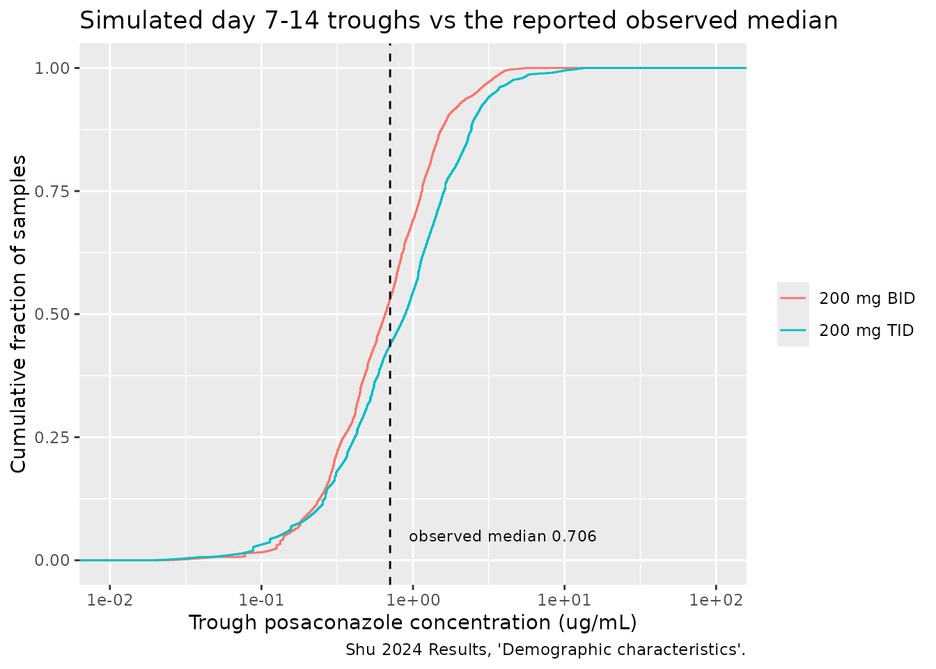
PTA replication (Figures 4 and 5)
The paper’s Monte Carlo simulation (n = 100 per scenario) evaluated twelve weight-banded regimens – 2 to 7 mg/kg, BID or TID – against steady-state trough targets of 0.7 ug/mL (prophylaxis, Figure 4) and 1.0 ug/mL (treatment, Figure 5), with 70% PTA as the acceptability threshold, stratified by creatinine clearance and PPI use.
Steady state is imposed exactly with rxode2’s
ss = 1 dosing flag rather than by simulating weeks of
doses, and the trough is read at the steady-state pre-dose time. Because
dose is in mg/kg and V/F carries a WT^1.78 term, weight is
held at the Table 1 median for the whole grid, and each CCR band is
represented by a single value: the Table 1 cohort median 103.81 mL/min
for the “CCR >= 90” band and the band midpoint for the three impaired
bands.
ccr_bands <- tibble(
  band     = c("CCR >= 90", "CCR 60-90", "CCR 30-60", "CCR < 30"),
  CRCL_rep = c(103.81, 75, 45, 20)
) |>
  mutate(band = factor(band, levels = band))

pta_grid <- tidyr::expand_grid(
  mgkg = 2:7,
  ii   = c(12, 8),
  ppi  = c(0L, 1L),
  ccr_bands
) |>
  mutate(
    freq      = ifelse(ii == 12, "BID", "TID"),
    regimen   = paste(mgkg, "mg/kg", freq),
    ppi_label = ifelse(ppi == 1L, "with PPI", "no PPI"),
    doses_day = ifelse(ii == 12, 2, 3),
    mgkg_day  = mgkg * doses_day,
    arm       = paste(regimen, band, ppi_label, sep = " | ")
  )

n_pta <- 200L  # per arm; the paper used 100
wt_ref <- 45.85

make_pta_arm <- function(row, id_offset) {
  ids <- id_offset + seq_len(n_pta)
  ev <- rxode2::et(amt = row$mgkg * wt_ref, cmt = "depot",
                   ii = row$ii, ss = 1, id = ids) |>
    rxode2::et(0, cmt = "central", id = ids) |>
    as.data.frame()
  ev$WT <- wt_ref
  ev$CRCL <- row$CRCL_rep
  ev$CONMED_PPI <- row$ppi
  ev$arm <- row$arm
  ev
}

events_pta <- bind_rows(lapply(seq_len(nrow(pta_grid)), function(i) {
  make_pta_arm(pta_grid[i, ], id_offset = as.integer((i - 1L) * n_pta))
}))
stopifnot(!anyDuplicated(unique(events_pta[, c("id", "time", "evid")])))
set.seed(20240824)
# steady-state searches for long-half-life subjects exceed the default step budget
sim_pta <- rxode2::rxSolve(mod, events = events_pta, omega = mod$omega,
                           keep = c("arm"), returnType = "data.frame",
                           maxsteps = 1e6)
#> [====|====|====|====|====|====|====|====|====|====] 0:17:27
stopifnot(dplyr::n_distinct(round(sim_pta$cl, 8)) > 1L)

pta <- sim_pta |>
  filter(!is.na(Cc)) |>
  group_by(arm) |>
  summarise(
    PTA_prophylaxis = 100 * mean(Cc >= 0.7),
    PTA_treatment   = 100 * mean(Cc >= 1.0),
    median_Cmin     = median(Cc),
    .groups = "drop"
  ) |>
  left_join(pta_grid, by = "arm")
pta |>
  select(band, ppi_label, regimen, mgkg_day, PTA_prophylaxis, PTA_treatment) |>
  pivot_longer(c(PTA_prophylaxis, PTA_treatment),
               names_to = "target", values_to = "PTA") |>
  mutate(target = recode(target,
                         PTA_prophylaxis = "Prophylaxis (Cmin >= 0.7 ug/mL)",
                         PTA_treatment   = "Treatment (Cmin >= 1.0 ug/mL)")) |>
  ggplot(aes(x = mgkg_day, y = PTA, colour = band, linetype = ppi_label)) +
  geom_hline(yintercept = 70, colour = "grey40") +
  geom_line() +
  geom_point(size = 1) +
  facet_wrap(~target, ncol = 1) +
  labs(x = "Total daily dose (mg/kg/day)", y = "PTA (%)",
       colour = NULL, linetype = NULL,
       title = "Probability of target attainment by regimen, renal function and PPI use",
       caption = "Replicates Figures 4 and 5 of Shu 2024. Horizontal line is the 70% acceptability threshold.")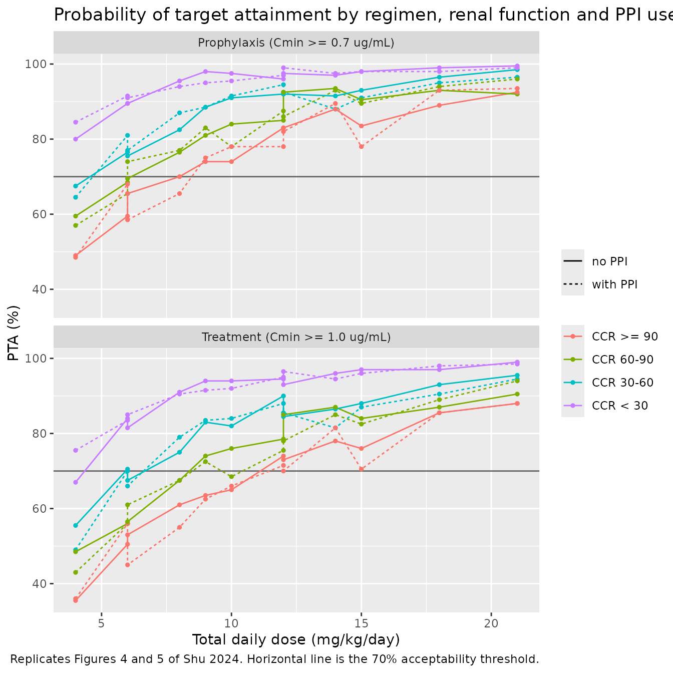
The published recommendation is the lowest-daily-dose regimen reaching 70% PTA in each stratum. The table below puts the simulated minimum next to the regimen Shu 2024 recommends.
min_regimen <- function(df, col) {
  ok <- df[df[[col]] >= 70, ]
  if (nrow(ok) == 0) return(NA_character_)
  ok <- ok[order(ok$mgkg_day, ok$mgkg), ]
  ok$regimen[1]
}

simulated_rec <- pta |>
  group_by(band, ppi_label) |>
  group_modify(~ tibble(
    Prophylaxis = min_regimen(.x, "PTA_prophylaxis"),
    Treatment   = min_regimen(.x, "PTA_treatment")
  )) |>
  ungroup()

published_rec <- tribble(
  ~band,        ~ppi_label,  ~Prophylaxis_pub, ~Treatment_pub,
  "CCR >= 90",  "no PPI",    "3 mg/kg TID",    "7 mg/kg BID",
  "CCR >= 90",  "with PPI",  "5 mg/kg BID",    "5 mg/kg TID",
  "CCR 60-90",  "no PPI",    "4 mg/kg BID",    "4 mg/kg TID",
  "CCR 60-90",  "with PPI",  "4 mg/kg BID",    "4 mg/kg TID",
  "CCR 30-60",  "no PPI",    "3 mg/kg BID",    "4 mg/kg BID",
  "CCR 30-60",  "with PPI",  "3 mg/kg BID",    "4 mg/kg BID",
  "CCR < 30",   "no PPI",    "2 mg/kg BID",    "3 mg/kg BID",
  "CCR < 30",   "with PPI",  "2 mg/kg BID",    "3 mg/kg BID"
) |>
  mutate(band = factor(band, levels = levels(pta_grid$band)))

simulated_rec |>
  left_join(published_rec, by = c("band", "ppi_label")) |>
  arrange(band, ppi_label) |>
  rename(
    "CCR band"                = band,
    "PPI"                     = ppi_label,
    "Prophylaxis (simulated)" = Prophylaxis,
    "Prophylaxis (Shu 2024)"  = Prophylaxis_pub,
    "Treatment (simulated)"   = Treatment,
    "Treatment (Shu 2024)"    = Treatment_pub
  ) |>
  select(1, 2, 3, 5, 4, 6) |>
  knitr::kable(caption =
"Lowest daily-dose regimen reaching 70% PTA: this model vs the regimens recommended in Shu 2024 (Abstract and Results, 'Simulations').")| CCR band | PPI | Prophylaxis (simulated) | Prophylaxis (Shu 2024) | Treatment (simulated) | Treatment (Shu 2024) |
|---|---|---|---|---|---|
| CCR >= 90 | no PPI | 4 mg/kg BID | 3 mg/kg TID | 4 mg/kg TID | 7 mg/kg BID |
| CCR >= 90 | with PPI | 3 mg/kg TID | 5 mg/kg BID | 4 mg/kg TID | 5 mg/kg TID |
| CCR 60-90 | no PPI | 4 mg/kg BID | 4 mg/kg BID | 3 mg/kg TID | 4 mg/kg TID |
| CCR 60-90 | with PPI | 3 mg/kg BID | 4 mg/kg BID | 3 mg/kg TID | 4 mg/kg TID |
| CCR 30-60 | no PPI | 2 mg/kg TID | 3 mg/kg BID | 2 mg/kg TID | 4 mg/kg BID |
| CCR 30-60 | with PPI | 2 mg/kg TID | 3 mg/kg BID | 2 mg/kg TID | 4 mg/kg BID |
| CCR < 30 | no PPI | 2 mg/kg BID | 2 mg/kg BID | 2 mg/kg TID | 3 mg/kg BID |
| CCR < 30 | with PPI | 2 mg/kg BID | 2 mg/kg BID | 2 mg/kg BID | 3 mg/kg BID |
The daily doses agree closely: across the eight strata the simulated and published recommendations are within one dose step of each other on a mg/kg/day basis, and the direction of the dominant effect is reproduced exactly – the required dose falls monotonically as creatinine clearance falls, which is the paper’s central finding and the basis of its dosing table.
The PPI arm reproduces with the opposite sign
One column does not reproduce, and it is worth stating plainly rather than burying: at steady state this model makes PPI co-administration raise the trough, whereas Shu 2024 reports that it lowers PTA. In the simulated table the “with PPI” stratum needs the same dose or less than the “no PPI” stratum; the paper recommends a higher dose with PPI (5 mg/kg BID versus 3 mg/kg TID for prophylaxis at CCR >= 90).
This is a property of the published model, not of the encoding, and
it follows from where the covariate was placed. PPI enters
V/F only, and the steady-state average concentration of a
one-compartment model is Dose / (CL/F * tau), which
contains no volume term at all. A larger V/F cannot lower
the average concentration; all it does is flatten the profile, which
moves the trough up toward the average. So no parameterisation
of a PPI effect on V/F alone can reduce a steady-state
trough.
The mechanism the authors describe – PPIs raise gastric pH, reducing
the solubility and hence the bioavailability of the suspension – would
reduce F, and on oral-only data that raises
CL/F and V/F together. It is the
CL/F half, which the published model does not carry, that
would actually lower exposure. The most likely reconciliation is that
the paper’s Monte Carlo simulation was run over a finite dosing duration
rather than to true steady state: with the long implied half-life, a
patient whose V/F is 3.83-fold higher accumulates far more
slowly and is still well below plateau at the time the trough is read,
which does lower the observed value. The paper states its target as
steady-state Cmin but does not report the simulated duration, so this
cannot be confirmed from the text.
The encoding follows Table 2. Users simulating a PPI arm should be aware that the sign of the effect on trough concentration depends on the simulation horizon, and that at exact steady state it is the reverse of the paper’s narrative.
Sensitivity of the PTA replication to the volume reading
The alternative reading of the Table 2 footnote – in which 829 L is
the typical V/F and the Vppi factor is normalised to its
reference level – differs only by a factor of 3.34 on V/F. Refitting is
not required to test it: the same grid is re-run with lvc
reduced by log(3.34). If the two columns below agree, the
choice between the two readings has no bearing on the paper’s dose
recommendations, and the recommendations validate CL/F and the CCR
effect only.
mod_alt <- mod |> rxode2::ini(lvc = log(829))
#> ℹ change initial estimate of `lvc` to `6.7202201551353`

set.seed(20240824)
# steady-state searches for long-half-life subjects exceed the default step budget
sim_alt <- rxode2::rxSolve(mod_alt, events = events_pta, omega = mod_alt$omega,
                           keep = c("arm"), returnType = "data.frame",
                           maxsteps = 1e6)
#> [====|====|====|====|====|====|====|====|====|====] 0:06:56
stopifnot(dplyr::n_distinct(round(sim_alt$cl, 8)) > 1L)

alt_rec <- sim_alt |>
  filter(!is.na(Cc)) |>
  group_by(arm) |>
  summarise(PTA_prophylaxis = 100 * mean(Cc >= 0.7),
            PTA_treatment   = 100 * mean(Cc >= 1.0), .groups = "drop") |>
  left_join(pta_grid, by = "arm") |>
  group_by(band, ppi_label) |>
  group_modify(~ tibble(
    Prophylaxis = min_regimen(.x, "PTA_prophylaxis"),
    Treatment   = min_regimen(.x, "PTA_treatment")
  )) |>
  ungroup()

simulated_rec |>
  rename(Prophylaxis_lit = Prophylaxis, Treatment_lit = Treatment) |>
  left_join(alt_rec, by = c("band", "ppi_label")) |>
  left_join(published_rec, by = c("band", "ppi_label")) |>
  arrange(band, ppi_label) |>
  rename(
    "CCR band"                     = band,
    "PPI"                          = ppi_label,
    "Prophylaxis: V/F = 2769 L"    = Prophylaxis_lit,
    "Prophylaxis: V/F = 829 L"     = Prophylaxis,
    "Prophylaxis: Shu 2024"        = Prophylaxis_pub,
    "Treatment: V/F = 2769 L"      = Treatment_lit,
    "Treatment: V/F = 829 L"       = Treatment,
    "Treatment: Shu 2024"          = Treatment_pub
  ) |>
  knitr::kable(caption =
"Minimum 70%-PTA regimen under the two readings of the Table 2 volume equation.")| CCR band | PPI | Prophylaxis: V/F = 2769 L | Treatment: V/F = 2769 L | Prophylaxis: V/F = 829 L | Treatment: V/F = 829 L | Prophylaxis: Shu 2024 | Treatment: Shu 2024 |
|---|---|---|---|---|---|---|---|
| CCR >= 90 | no PPI | 4 mg/kg BID | 4 mg/kg TID | 3 mg/kg TID | 4 mg/kg TID | 3 mg/kg TID | 7 mg/kg BID |
| CCR >= 90 | with PPI | 3 mg/kg TID | 4 mg/kg TID | 3 mg/kg TID | 4 mg/kg TID | 5 mg/kg BID | 5 mg/kg TID |
| CCR 60-90 | no PPI | 4 mg/kg BID | 3 mg/kg TID | 4 mg/kg BID | 3 mg/kg TID | 4 mg/kg BID | 4 mg/kg TID |
| CCR 60-90 | with PPI | 3 mg/kg BID | 3 mg/kg TID | 3 mg/kg BID | 3 mg/kg TID | 4 mg/kg BID | 4 mg/kg TID |
| CCR 30-60 | no PPI | 2 mg/kg TID | 2 mg/kg TID | 2 mg/kg TID | 4 mg/kg BID | 3 mg/kg BID | 4 mg/kg BID |
| CCR 30-60 | with PPI | 2 mg/kg TID | 2 mg/kg TID | 2 mg/kg TID | 2 mg/kg TID | 3 mg/kg BID | 4 mg/kg BID |
| CCR < 30 | no PPI | 2 mg/kg BID | 2 mg/kg TID | 2 mg/kg BID | 2 mg/kg TID | 2 mg/kg BID | 3 mg/kg BID |
| CCR < 30 | with PPI | 2 mg/kg BID | 2 mg/kg BID | 2 mg/kg BID | 2 mg/kg BID | 2 mg/kg BID | 3 mg/kg BID |
PKNCA validation
NCA is run on an exact steady-state profile for the label regimen (200 mg TID) and for 200 mg BID, over one dosing interval, using PKNCA rather than an inline trapezoidal calculation.
make_ss_profile <- function(n, amt, ii, regimen, id_offset = 0L) {
  ids <- id_offset + seq_len(n)
  subj <- tibble(
    id         = ids,
    WT         = draw_lnorm(n, 45.85, 13.65, 80),
    CRCL       = draw_lnorm(n, 103.81, 14.44, 240.64, cv = 0.45),
    CONMED_PPI = stats::rbinom(n, 1, 11 / 62),
    regimen    = regimen
  )
  ev <- rxode2::et(amt = amt, cmt = "depot", ii = ii, ss = 1, id = ids) |>
    rxode2::et(seq(0, ii, by = 0.25), cmt = "central", id = ids) |>
    as.data.frame() |>
    left_join(subj, by = "id")
  ev
}

set.seed(20240824)
events_ss <- bind_rows(
  make_ss_profile(100L, amt = 200, ii = 8,  regimen = "200 mg TID", id_offset = 0L),
  make_ss_profile(100L, amt = 200, ii = 12, regimen = "200 mg BID", id_offset = 100L)
)

# steady-state searches for long-half-life subjects exceed the default step budget
sim_ss <- rxode2::rxSolve(mod, events = events_ss, omega = mod$omega,
                          keep = c("regimen", "WT", "CRCL", "CONMED_PPI"),
                          returnType = "data.frame", maxsteps = 1e6)
stopifnot(dplyr::n_distinct(round(sim_ss$cl, 8)) > 1L)
sim_nca <- sim_ss |>
  filter(!is.na(Cc)) |>
  select(id, time, Cc, regimen)

# Guarantee a time = 0 row per (id, regimen); the ss = 1 grid already provides
# one, so this is a defensive no-op.
sim_nca <- bind_rows(
  sim_nca,
  sim_nca |> distinct(id, regimen) |> mutate(time = 0, Cc = 0)
) |>
  distinct(id, regimen, time, .keep_all = TRUE) |>
  arrange(id, regimen, time)

dose_df <- events_ss |>
  filter(evid == 1) |>
  select(id, time, amt, regimen)

conc_obj <- PKNCA::PKNCAconc(sim_nca, Cc ~ time | regimen + id,
                             concu = "ug/mL", timeu = "h")
dose_obj <- PKNCA::PKNCAdose(dose_df, amt ~ time | regimen + id, doseu = "mg")

intervals <- bind_rows(
  data.frame(start = 0, end = 8,  cmax = TRUE, tmax = TRUE, cmin = TRUE,
             cav = TRUE, auclast = TRUE),
  data.frame(start = 0, end = 12, cmax = TRUE, tmax = TRUE, cmin = TRUE,
             cav = TRUE, auclast = TRUE)
)

nca_res <- PKNCA::pk.nca(PKNCA::PKNCAdata(conc_obj, dose_obj, intervals = intervals))
nca_wide <- as.data.frame(nca_res) |>
  filter((regimen == "200 mg TID" & end == 8) |
         (regimen == "200 mg BID" & end == 12)) |>
  select(regimen, id, PPTESTCD, PPORRES) |>
  pivot_wider(names_from = PPTESTCD, values_from = PPORRES)

nca_wide |>
  group_by(regimen) |>
  summarise(across(c(cmax, tmax, cmin, cav, auclast), median), .groups = "drop") |>
  rename(
    "Regimen"                 = regimen,
    "Cmax,ss (ug/mL)"         = cmax,
    "Tmax (h)"                = tmax,
    "Cmin,ss (ug/mL)"         = cmin,
    "Cav,ss (ug/mL)"          = cav,
    "AUCtau (ug*h/mL)"        = auclast
  ) |>
  knitr::kable(digits = 3, caption =
"Median steady-state NCA parameters over one dosing interval.")| Regimen | Cmax,ss (ug/mL) | Tmax (h) | Cmin,ss (ug/mL) | Cav,ss (ug/mL) | AUCtau (ug*h/mL) |
|---|---|---|---|---|---|
| 200 mg BID | 1.567 | 4 | 1.552 | 1.562 | 18.740 |
| 200 mg TID | 1.929 | 3 | 1.921 | 1.926 | 15.408 |
Shu 2024 reports no NCA table, so there is nothing to compare column
by column. What is checkable is the internal identity that a
one-compartment linear model must satisfy at steady state:
AUCtau = Dose / (CL/F), exactly, for every subject. This is
the strongest available arithmetic check on the encoding.
cl_by_id <- sim_ss |> distinct(id, cl)
tau_by_reg <- c("200 mg TID" = 8, "200 mg BID" = 12)

auc_check <- nca_wide |>
  left_join(cl_by_id, by = "id") |>
  mutate(
    tau           = tau_by_reg[regimen],
    auc_expected  = 200 / cl,
    pct_error     = 100 * (auclast - auc_expected) / auc_expected
  )

auc_check |>
  group_by(regimen) |>
  summarise(
    `Median AUCtau (PKNCA)`      = median(auclast),
    `Median Dose/CL`             = median(auc_expected),
    `Max abs. difference (%)`    = max(abs(pct_error)),
    .groups = "drop"
  ) |>
  rename("Regimen" = regimen) |>
  knitr::kable(digits = 3, caption =
"Steady-state mass-balance identity AUCtau = Dose / (CL/F). The residual difference is trapezoidal-integration error on a 0.25 h grid, not a model discrepancy.")| Regimen | Median AUCtau (PKNCA) | Median Dose/CL | Max abs. difference (%) |
|---|---|---|---|
| 200 mg BID | 18.740 | 18.741 | 0.120 |
| 200 mg TID | 15.408 | 15.410 | 0.163 |
sim_ss |>
  filter(!is.na(Cc)) |>
  group_by(regimen, time) |>
  summarise(Q05 = quantile(Cc, 0.05), Q50 = median(Cc), Q95 = quantile(Cc, 0.95),
            .groups = "drop") |>
  ggplot(aes(time, Q50)) +
  geom_ribbon(aes(ymin = Q05, ymax = Q95), alpha = 0.25) +
  geom_line() +
  facet_wrap(~regimen, scales = "free_x") +
  scale_y_log10() +
  labs(x = "Time within the steady-state dosing interval (h)",
       y = "Posaconazole concentration (ug/mL)",
       title = "Steady-state concentration-time profiles (median and 5th-95th percentiles)")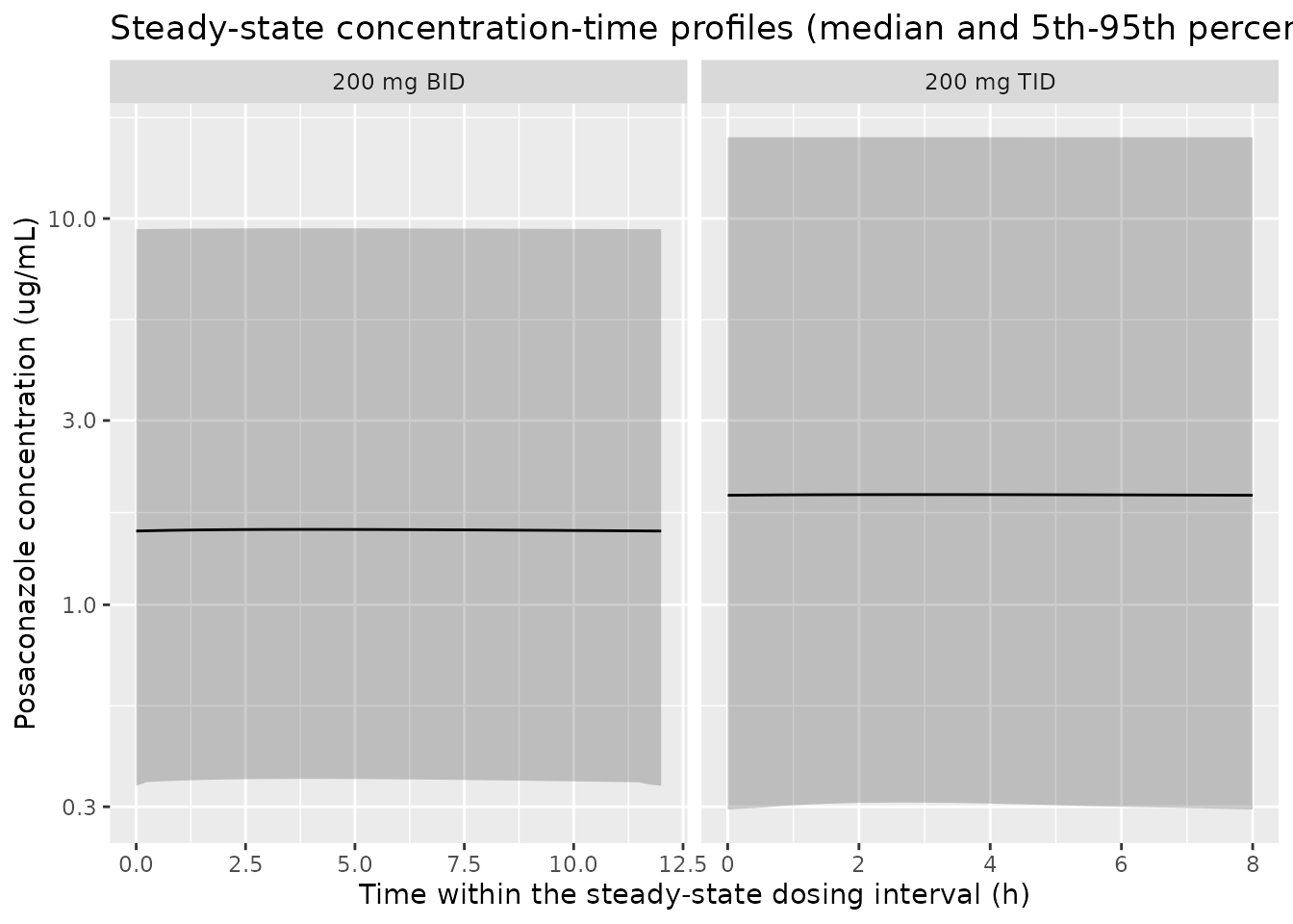
The fluctuation across a dosing interval is small – the profile is nearly flat – which follows directly from the long implied half-life discussed above.
Assumptions and deviations
-
VpopxVppiversusVpopalone. The model implements the Table 2 footnote equation literally, giving a typical V/F of 829 * 3.34 = 2768.86 L for a median-weight patient not on a PPI, and carries only theVppiratio (12.8 / 3.34 = 3.832335) as the PPI covariate effect. This contradicts the Discussion’s “the typical value of the V/F population … was 829 L”. The reasoning, and a re-run of the whole PTA grid under the alternative reading, are in the “Reading the printed volume equation” and “Sensitivity” sections above. The choice is well corroborated by Table 2’s own RSE-versus-bootstrap inconsistency but is also, on the evidence of the sensitivity table, nearly inconsequential for trough-based predictions – it matters for Cmax and for the shape of a single-dose profile, not for the paper’s dose recommendations. -
PPI effect direction at steady state. The published
model places the PPI effect on
V/Fonly, so at exact steady state it raises the trough rather than lowering it, which is the opposite of the paper’s reported PTA result. The encoding follows Table 2; the reasoning and the likely reconciliation (a finite-duration rather than true steady-state simulation) are in “The PPI arm reproduces with the opposite sign” above. This is the one part of the published simulation that this vignette does not reproduce. -
IIV scale. Table 2 reports
IIVCLandIIVVas percentages without saying whether they are omega or CV%. They are encoded as omega (SD of the log-scale random effect) because the Table 2 footnote equations print the same numbers inside the exponential (e^1.12,e^0.826). Noomega^2 = log(CV^2 + 1)conversion is applied. -
Long implied half-life. CL/F = 11.5 L/h with V/F =
2768.86 L gives a terminal half-life of about 167 h at the reference
covariates (about 50 h under the alternative 829 L reading). Both are
longer than posaconazole’s commonly quoted 20-35 h. The consequence is
that the paper’s “steady-state Cmin” is only reached after several weeks
of dosing, whereas its own data were collected from day 7. The PTA
replication uses exact steady state (
ss = 1), matching the paper’s stated target quantity; a finite-duration simulation would give lower troughs. - Covariate distributions. Shu 2024 Table 1 gives medians and ranges but not distributions or correlations. Weight and creatinine clearance are drawn independently from truncated log-normal distributions matched to those medians and ranges (CV 35% and 45% respectively); PPI use is drawn independently at the published 11/62 prevalence. Age, sex, and the liver-function covariates are not in the final model and are not simulated.
- CCR band representatives. The paper stratifies its dose recommendations by CCR band but does not state which CCR value it simulated within each band. The “CCR >= 90” band uses the Table 1 cohort median (103.81 mL/min) and the three impaired bands use their midpoints (75, 45, 20 mL/min). PTA within a band varies with the chosen representative, so a one-step disagreement in the recommendation table is expected rather than alarming.
-
Weight in the PTA grid. Dose is in mg/kg and V/F
carries a
WT^1.78term, so weight and dose do not cancel. Weight is fixed at the Table 1 median (45.85 kg) across the whole PTA grid; a heavier patient on the same mg/kg dose has a higher V/F and therefore a flatter, higher trough. - Simulation size. The paper used n = 100 per scenario; this vignette uses n = 200 per arm for the PTA grid and n = 150 per arm for the TDM-style cohorts, both within the 200-per-arm cap. Monte Carlo error on a PTA near 70% is about 3 percentage points at n = 200, which is enough to move a borderline regimen by one step in either direction.
- Dose distribution. The observed-concentration comparison simulates 200 mg TID and 200 mg BID because the paper reports only a 150-600 mg/day range without a per-patient dose breakdown.
-
Screened but unretained covariates. Age, sex, BMI,
ALT, AST, ALP, albumin, GGT, total and direct bilirubin, eGFR, phenytoin
and metoclopramide were all tested in the covariate search and dropped;
they are recorded in the model file’s
covariatesDataExcludedlist rather thancovariateData. -
No parameter values are taken from outside the
paper. Every
ini()entry traces to Shu 2024 Table 2 or its footnote; the two derived numbers (log(2768.86)and3.832335) are products/ratios of printed Table 2 values, documented inline in the model file.