Model and source
ui <- rxode2::rxode(readModelDb("Edrich_2015_heparin"))- Citation: Edrich T, Frendl G, Michaud G, Paschalidis ICh. Heparin requirements for full anticoagulation are higher for patients on dabigatran than for those on warfarin - a model-based study. Clin Pharmacol. 2015;7:19-27. doi:10.2147/CPAA.S72185.
- Article: https://doi.org/10.2147/CPAA.S72185 (open access; PMC4327399)
- Description: One-compartment population PK + linear direct-effect PD model for intravenous heparin in adults undergoing catheter-based ablation of atrial fibrillation (Edrich 2015). Because only heparin doses and the resulting activated clotting times (ACT) were recorded, the PK and PD layers are not separately identifiable: the central compartment holds heparin units in the estimated blood volume and a single multiplicative sensitivity coefficient k_ACT maps that scaled concentration onto the ACT in seconds, ACT = ACT_BASE + k_ACT * Cc. The central volume is not estimated but set to the weight-based estimated blood volume, which is sex-dependent. k_ACT carries a four-level multiplicative factor for the patient’s chronic oral anticoagulant at presentation (none = reference; warfarin with INR < 2; warfarin with INR >= 2; dabigatran stopped about 27 h earlier), which is the paper’s finding: warfarin patients are about twice as heparin-sensitive as dabigatran or unanticoagulated patients. Clearance carried no group effect in the final model. The point-of-care instrument ceiling of 400 s is NOT applied to the prediction here (it is an estimation device in the source control stream, not pharmacology); see the vignette for its consequences.
Edrich 2015 asks a narrow, practical question: when a patient who has been on a chronic oral anticoagulant presents for catheter-based ablation of atrial fibrillation, how much intravenous heparin do they need to reach full anticoagulation? The answer, from a one-compartment PK/PD model fitted to 188 patients’ complete intraprocedural anticoagulation courses, is that patients on warfarin are roughly twice as heparin-sensitive as patients on dabigatran or on no chronic anticoagulant at all, and that dabigatran withheld for about two half-lives leaves heparin sensitivity indistinguishable from no anticoagulation.
Two features of the source shape everything below.
The PK and PD layers are not separately
identifiable. Only heparin doses and the resulting activated
clotting times (ACT) were recorded; plasma heparin was never assayed.
The model therefore fixes the central volume to the weight-based
estimated blood volume and lets a single multiplicative
coefficient k_ACT carry everything between the scaled
concentration and the ACT:
Cc in the packaged model is that scaled concentration
(heparin units per litre of blood volume) and carries no
residual error, because it was never measured. ACT
is the only observed endpoint.
The final parameter estimates are never tabulated.
The supplement prints the complete NONMEM 7 control stream, but its
$THETA / $OMEGA / $SIGMA blocks
are starting values in LOWER STARTING UPPER form.
Every structural value in the packaged model is therefore recovered from
the paper’s reported results, and each recovered value is then checked
against the corresponding control-stream bound as an independent
consistency test. All of them pass, and one of them –
THETA(3) – passes only just, which is what makes the check
informative. See Recovering the final estimates below.
Population
188 adults with atrial fibrillation presenting for catheter-based
atrial ablation at Brigham and Women’s Hospital between January 2011 and
June 2012, identified by retrospective chart review (IRB-approved,
written consent waived). Patients were grouped by their chronic oral
anticoagulant at presentation: dabigatran (group D, n = 66), warfarin
(group W, n = 95) and no chronic anticoagulant (group N, n = 27). Group
W was subdivided by the last pre-procedural INR into W_low
(INR < 2, an unintentionally low value, n = 42) and
W_high (INR >= 2 within the last 3 days, n = 53).
Table 1 of the source gives median age 58-64 years by group, median BMI 26.3-29.3 kg/m^2, 63-71% male and 81-95% Caucasian; the paper found no significant difference in any model parameter by race. The last dose of the chronic anticoagulant preceded the procedure by a median 27 h (IQR 24-31) in group D and 15 h in both warfarin groups. Heparin dosing was not standardized: each patient received a median of three intravenous boluses and six ACT measurements per case, with no infusions.
All ACT values were measured on a Hemochron Signature Elite
whole-blood microcoagulation system with a Hemochron Jr cartridge,
measurement range 0-400 s. That ceiling matters: the first post-heparin
ACT exceeded 400 s in 69%, 77%, 24% and 7% of the W_low,
W_high, D and N groups respectively, so the group-W entries
of Table 2 are right-censored and understate the true
response. The paper says so explicitly in its Discussion, and the
validation below both relies on and confirms that reading.
The same information is available programmatically via
rxode2::rxode(readModelDb("Edrich_2015_heparin"))$population.
str(ui$population, max.level = 1, give.attr = FALSE)
#> List of 16
#>  $ species                  : chr "human"
#>  $ n_subjects               : int 188
#>  $ n_studies                : int 1
#>  $ age_median               : chr "64 y (dabigatran), 58 y (warfarin INR < 2), 62 y (warfarin INR >= 2), 58 y (no anticoagulant); Table 1 medians"
#>  $ weight_range             : chr "Not reported. Table 1 gives BMI only (medians 29.3, 28.7, 29.3, 26.3 kg/m^2 by group); see covariateData[['WT']]$notes"
#>  $ bmi_range                : chr "Group medians 26.3-29.3 kg/m^2 (Table 1)"
#>  $ sex_female_pct           : num 31.5
#>  $ race_ethnicity           : chr "Caucasian 94% (dabigatran), 95% (warfarin INR < 2), 94% (warfarin INR >= 2), 81% (no anticoagulant) per Table 1"| __truncated__
#>  $ disease_state            : chr "Adults with atrial fibrillation presenting for catheter-based atrial ablation requiring full intraprocedural an"| __truncated__
#>  $ dose_range               : chr "Not reported. Heparin dosing was not standardized in this retrospective cohort; each patient received a median "| __truncated__
#>  $ regions                  : chr "Single-centre: Brigham and Women's Hospital, Boston, MA, USA (IRB-approved retrospective chart review, January "| __truncated__
#>  $ n_group_dabigatran       : int 66
#>  $ n_group_warfarin_inr_low : int 42
#>  $ n_group_warfarin_inr_high: int 53
#>  $ n_group_no_anticoagulant : int 27
#>  $ notes                    : chr "Baseline demographics from Edrich 2015 Table 1. Group W (warfarin, n = 95) was subdivided by the last pre-proce"| __truncated__
Source trace
Every ini() entry carries its origin as an in-file
comment in
inst/modeldb/specificDrugs/Edrich_2015_heparin.R. Collected
here for review:
| Equation / parameter | Value | Source location |
|---|---|---|
d/dt(central) <- -kel * central |
n/a | Supplement $PK: K = CL/V1, ADVAN1
one-compartment |
vc <- c_sex * WT |
n/a | Supplement $PK:
V1 = (0.075 - 0.005*(M1F2-1))*WT*(1 + THETA(6))
|
Cc <- central / vc |
n/a | Supplement $PK: S1 = V1;
$ERROR comment names F as a scaled
concentration in “Units heparin/L blood volume” |
groupmod |
n/a | Supplement $PK:
GROUPMOD = NEITHER*1 + COUMLO*THETA(3) + COUMHI*THETA(4) + PRADAX*THETA(5)
|
ACT <- ACT_BASE + slope * Cc |
n/a | Supplement $ERROR:
Predicted_ACT = F*KACT + BASEACT
|
lcl |
23.9 mL/min | Results: group medians of individual CL 22.4 / 22.1 / 26.5 / 23.4 mL/min; n-weighted mean. No group term on CL in the final model |
lvc_male |
0.075 L/kg | Supplement $PK numeric literal,
M1F2 = 1
|
lvc_female |
0.070 L/kg | Supplement $PK numeric literal,
M1F2 = 2
|
lslope |
0.12 s*L/IU | Table 3: median individual k_ACT, group N (the
GROUPMOD reference) |
e_warflo_slope |
0.23 / 0.12 = 1.92 | Table 3: group W_low median / group N median |
e_warfhi_slope |
0.30 / 0.12 = 2.50 | Table 3: group W_high median / group N median |
e_dabigatran_slope |
0.13 / 0.12 = 1.08 | Table 3: group D median / group N median |
propSd |
0.153 | Results: final-model RMS error 51.1 ACT-seconds = 15.3% of the average ACT |
addSd |
0 | Supplement $SIGMA(2) declares an additive component;
final value not reported |
ACT_BASE (covariate) |
144 / 155 / 169 / 182 s | Table 1, group medians of pre-heparin ACT |
INR_BASE (covariate) |
1.0 / 1.2 / 1.8 / 2.3 | Results and Table 1, group means of the last pre-procedural INR |
WT (covariate) |
not tabulated | Back-solved below from the printed half-life range and group clearances |
IIV ($OMEGA BLOCK(2)) |
not reported | Starting values only; typical-value model, no etas |
Recovering the final estimates
The reference group is unambiguous: the control stream’s own comment
reads group "neither" is the reference == 1, so
THETA(2) is the group-N k_ACT and
THETA(3)-THETA(5) are ratios to it. The
recovered values are then checked against the control stream’s own
$THETA bounds – a test the authors did not intend to
provide, and which the reference-group reading has to pass.
recovered <- tibble::tribble(
  ~theta,      ~quantity,                       ~value,             ~lower, ~upper,
  "THETA(1)",  "CL (L/min), pooled",            23.9 / 1000,        0,      10,
  "THETA(2)",  "k_ACT, group N reference",      0.12,               0,      20,
  "THETA(3)",  "multiplier, W_low",             0.23 / 0.12,        1,      2,
  "THETA(4)",  "multiplier, W_high",            0.30 / 0.12,        1,      4,
  "THETA(5)",  "multiplier, D",                 0.13 / 0.12,        0.6,    1.5
) |>
  mutate(`within bound` = value > lower & value < upper)

recovered |>
  mutate(value = signif(value, 4)) |>
  rename(
    "NONMEM theta" = theta, "Recovered quantity" = quantity,
    "Recovered value" = value, "Lower" = lower, "Upper" = upper
  ) |>
  knitr::kable(
    caption = paste(
      "Values recovered from the paper's Results / Table 3, checked against",
      "the supplement's own $THETA bounds. THETA(3) = 1.92 against an upper",
      "bound of 2 is the tightest fit and is the strongest single piece of",
      "evidence that group N is the GROUPMOD reference."
    )
)| NONMEM theta | Recovered quantity | Recovered value | Lower | Upper | within bound |
|---|---|---|---|---|---|
| THETA(1) | CL (L/min), pooled | 0.0239 | 0.0 | 10.0 | TRUE |
| THETA(2) | k_ACT, group N reference | 0.1200 | 0.0 | 20.0 | TRUE |
| THETA(3) | multiplier, W_low | 1.9170 | 1.0 | 2.0 | TRUE |
| THETA(4) | multiplier, W_high | 2.5000 | 1.0 | 4.0 | TRUE |
| THETA(5) | multiplier, D | 1.0830 | 0.6 | 1.5 | TRUE |
Back-solving the cohort’s typical body weight
The paper never tabulates body weight – Table 1 reports BMI only –
yet weight sets the central volume and hence the elimination rate
constant. It is nonetheless recoverable from quantities the paper
does print. Results gives the per-group median clearances and
states that “the corresponding half-lives of the effect of heparin on
the ACT ranged from 154 minutes to 180 minutes”. Since
t_half = ln(2) * V1 / CL and V1 = 0.075 * WT
for a male, the longest half-life must pair with the smallest clearance
and the shortest with the largest:
cl_group <- c(W_low = 22.4, W_high = 22.1, D = 26.5, N = 23.4) / 1000 # L/min
vc_per_kg_male <- 0.075                                              # L/kg

wt_from_thalf <- function(t_half, cl) t_half * cl / (log(2) * vc_per_kg_male)

wt_candidates <- c(
  `longest t_half (180 min) with smallest CL` = wt_from_thalf(180, min(cl_group)),
  `shortest t_half (154 min) with largest CL` = wt_from_thalf(154, max(cl_group))
)
print(round(wt_candidates, 1))
#> longest t_half (180 min) with smallest CL
#>                                      76.5
#> shortest t_half (154 min) with largest CL
#>                                      78.5

wt_typical <- round(mean(wt_candidates))
cat("Back-solved cohort-typical body weight:", wt_typical, "kg\n")
#> Back-solved cohort-typical body weight: 78 kg

# Physiological plausibility, not a test of the model: an adult cohort with a
# median BMI near 29 kg/m^2 must land in a broad but finite weight band. This
# gate is deliberately wide -- its job is to catch a unit error or an inverted
# pairing, not to certify the value.
stopifnot(wt_typical > 55, wt_typical < 110)
This is a derivation, not an independent validation: it consumes the printed half-life range, so “the model’s half-life falls in that range” is near-circular and is reported below as a consistency check rather than a test. The genuinely independent gates are the Table 2 and Table 3 reproductions.
One observation worth recording. At 78 kg and a median BMI of about 29 kg/m^2, the implied height is about 1.64 m, which is short for a cohort that is 63-71% male. The alternative blood-volume reading discussed in Errata below (70 mL/kg rather than 75 mL/kg for men) would back-solve to about 84 kg and an implied height near 1.70 m, which fits the demographics better. That is a soft, assumption-laden signal and it does not override the adopted reading, but it is the third independent hint pointing the same way and it belongs on the record.
Virtual cohort
The original patient-level data are not public. The cohort below reproduces the group structure, group sizes (scaled down), sex balance and baseline ACT of Table 1, and assigns body weights around the value back-solved above.
# Seeds R's RNG only. The packaged model declares NO eta terms, so rxSolve is
# fully deterministic given these covariates -- there is no rxode2 RNG stream
# involved and no thread-count dependence in anything below.
set.seed(20150219)

n_per_arm <- 50L # well under the 200-per-arm cap; the model has no IIV to average out

groups <- tibble::tribble(
  ~group,   ~CONMED_WARFARIN, ~CONMED_DABIGATRAN, ~INR_BASE, ~ACT_BASE, ~pct_male, ~n_source,
  "N",      0,                0,                  1.0,       144,       69,        27L,
  "D",      0,                1,                  1.2,       155,       71,        66L,
  "W_low",  1,                0,                  1.8,       169,       71,        42L,
  "W_high", 1,                0,                  2.3,       182,       63,        53L
)

make_arm <- function(row, id_offset) {
  tibble(
    id = id_offset + seq_len(n_per_arm),
    group = row$group,
    CONMED_WARFARIN = row$CONMED_WARFARIN,
    CONMED_DABIGATRAN = row$CONMED_DABIGATRAN,
    INR_BASE = row$INR_BASE,
    ACT_BASE = row$ACT_BASE,
    # Weight distribution is ASSUMED (see Assumptions): lognormal, median at
    # the back-solved typical weight, 15% CV -- a plausible adult spread. The
    # paper reports no weight distribution to match.
    WT = wt_typical * exp(stats::rnorm(n_per_arm, 0, 0.15)),
    SEXF = as.numeric(stats::runif(n_per_arm) > row$pct_male / 100)
  )
}

subjects <- do.call(
  rbind,
  lapply(seq_len(nrow(groups)), function(i) {
    make_arm(groups[i, ], id_offset = (i - 1L) * n_per_arm)
  })
)
# `group` is kept as a plain character column throughout: rxSolve(keep=) may
# return a factor column as character, so factor levels are re-applied after
# each solve rather than relied upon across one.
group_levels <- groups$group

stopifnot(
  nrow(subjects) == n_per_arm * nrow(groups),
  !anyDuplicated(subjects$id)
)

subjects |>
  mutate(group = factor(group, levels = group_levels)) |>
  group_by(group) |>
  summarise(
    n = dplyr::n(),
    `median WT (kg)` = round(median(WT), 1),
    `% female` = round(100 * mean(SEXF)),
    `ACT_BASE (s)` = median(ACT_BASE),
    .groups = "drop"
  ) |>
knitr::kable(caption = "Virtual cohort by chronic-anticoagulant group.")| group | n | median WT (kg) | % female | ACT_BASE (s) |
|---|---|---|---|---|
| N | 50 | 76.4 | 32 | 144 |
| D | 50 | 76.4 | 22 | 155 |
| W_low | 50 | 80.5 | 44 | 169 |
| W_high | 50 | 79.3 | 40 | 182 |
Replicating Table 3: the group effect on heparin sensitivity
Table 3 is the paper’s central result. It reports the median of the
individual k_ACT values by group; the packaged model
carries the group N value as lslope and the other three as
multiplicative covariate effects, so the reproduction is exact by
construction and the test is that the arithmetic and the group-indicator
logic are wired correctly.
# A single dose + one observation is enough to read the model's derived `slope`
# per subject; the group indicators are exercised on the way.
ev_probe <- subjects |>
  tidyr::crossing(tibble(time = c(0, 1), evid = c(1, 0), amt = c(1000, NA_real_))) |>
  filter((time == 0 & evid == 1) | (time == 1 & evid == 0)) |>
  mutate(cmt = "central") |> # ODE state name, never the observable "ACT"
  arrange(id, time, dplyr::desc(evid))

sim_probe <- rxode2::rxSolve(
  ui, ev_probe,
  keep = c("group", "WT", "SEXF", "ACT_BASE"),
  returnType = "data.frame", addDosing = FALSE
)
#> Warning: multi-subject simulation without without 'omega'

kact_model <- sim_probe |>
  mutate(group = as.character(group)) |>
  group_by(group) |>
  summarise(k_ACT_model = median(slope), spread = diff(range(slope)), .groups = "drop")

# slope depends only on the group indicators, so it must be constant within a
# group; if it is not, the indicator logic is wrong.
stopifnot(nrow(kact_model) == 4L, max(kact_model$spread) < 1e-12)
kact_model$spread <- NULL

published_kact <- tibble::tribble(
  ~group,   ~k_ACT_paper, ~iqr_lo, ~iqr_hi,
  "N",      0.12,         0.09,    0.14,
  "D",      0.13,         0.12,    0.16,
  "W_low",  0.23,         0.22,    0.25,
  "W_high", 0.30,         0.29,    0.33
)

tab3 <- kact_model |>
  left_join(published_kact, by = "group") |>
  mutate(`abs diff` = abs(k_ACT_model - k_ACT_paper))

tab3 |>
  mutate(`IQR (paper)` = sprintf("%.2f-%.2f", iqr_lo, iqr_hi)) |>
  select(group, k_ACT_model, k_ACT_paper, `IQR (paper)`, `abs diff`) |>
  rename(
    "Group" = group,
    "k_ACT model (s*L/IU)" = k_ACT_model,
    "k_ACT paper median" = k_ACT_paper
  ) |>
  knitr::kable(
    digits = 4,
    caption = "Replicates Table 3 of Edrich 2015: the PKPD coefficient k_ACT by chronic-anticoagulant group."
)| Group | k_ACT model (s*L/IU) | k_ACT paper median | IQR (paper) | abs diff |
|---|---|---|---|---|
| D | 0.13 | 0.13 | 0.12-0.16 | 0 |
| N | 0.12 | 0.12 | 0.09-0.14 | 0 |
| W_high | 0.30 | 0.30 | 0.29-0.33 | 0 |
| W_low | 0.23 | 0.23 | 0.22-0.25 | 0 |
Replicating Table 2: ACT response to the first heparin bolus
Table 2 is an independent summary: it was computed directly from the observed data by a non-parametric route (Kruskal-Wallis on the raw ratio), before any model was fitted. Reproducing it from the fitted model is therefore a genuine out-of-sample test of the whole chain.
The paper’s metric is the ACT increase per unit of heparin per kg of
body weight, read from the ACT drawn a median 31 minutes after the first
bolus. In this model that metric is dose-invariant:
ACT - ACT_BASE is linear in dose, so dividing by dose per
kg cancels the dose entirely. The absolute dose below is therefore an
arbitrary scale with no effect on the comparison, which matters because
the paper does not report the administered amounts.
dose_per_kg <- 100 # arbitrary scale; the metric below is dose-invariant
t_first_act <- 31 # Results: median 31 min (IQR 23-42) to the first post-bolus ACT

ev_bolus <- bind_rows(
  subjects |> mutate(time = 0, evid = 1L, amt = dose_per_kg * WT, cmt = "central"),
  subjects |>
    tidyr::crossing(tibble(time = c(t_first_act, 23, 42))) |>
    mutate(evid = 0L, amt = NA_real_, cmt = "central")
) |>
  arrange(id, time, dplyr::desc(evid))

sim_bolus <- rxode2::rxSolve(
  ui, ev_bolus,
  keep = c("group", "WT", "SEXF", "ACT_BASE"),
  returnType = "data.frame", addDosing = FALSE
) |>
  mutate(dACT_per_U_per_kg = (ACT - ACT_BASE) / dose_per_kg)
#> Warning: multi-subject simulation without without 'omega'

# Dose-invariance is a structural claim about the model; check it rather than
# asserting it in prose.
sim_check <- rxode2::rxSolve(
  ui,
  ev_bolus |> mutate(amt = ifelse(evid == 1L, 4 * amt, amt)),
  keep = c("group", "ACT_BASE"), returnType = "data.frame", addDosing = FALSE
) |>
  mutate(dACT_per_U_per_kg = (ACT - ACT_BASE) / (4 * dose_per_kg))
#> Warning: multi-subject simulation without without 'omega'
stopifnot(max(abs(sim_check$dACT_per_U_per_kg - sim_bolus$dACT_per_U_per_kg)) < 1e-9)

published_t2 <- tibble::tribble(
  ~group,   ~paper_median, ~iqr_lo, ~iqr_hi, ~pct_censored,
  "N",      1.4,           1.0,     1.7,     7,
  "D",      1.6,           1.3,     2.1,     24,
  "W_low",  2.5,           2.1,     3.1,     69,
  "W_high", 2.8,           2.5,     3.2,     77
)

tab2 <- sim_bolus |>
  filter(time == t_first_act) |>
  mutate(group = as.character(group)) |>
  group_by(group) |>
  summarise(model_median = median(dACT_per_U_per_kg), .groups = "drop") |>
  left_join(published_t2, by = "group") |>
  mutate(
    `in paper IQR` = model_median >= iqr_lo & model_median <= iqr_hi,
    `pct diff vs median` = round(100 * (model_median / paper_median - 1), 1)
  )

tab2 |>
  mutate(
    `paper median (IQR)` = sprintf("%.1f (%.1f-%.1f)", paper_median, iqr_lo, iqr_hi),
    model_median = round(model_median, 2)
  ) |>
  select(group, model_median, `paper median (IQR)`, `in paper IQR`, `pct diff vs median`, pct_censored) |>
  rename(
    "Group" = group,
    "Model (dACT per IU per kg)" = model_median,
    "Paper median (IQR)" = `paper median (IQR)`,
    "% >400 s in source" = pct_censored
  ) |>
  knitr::kable(
    caption = paste(
      "Replicates Table 2 of Edrich 2015: ACT response to the first heparin",
      "bolus, at the paper's median 31 min sampling time. The last column is",
      "the fraction of that group's first post-heparin ACTs that exceeded the",
      "instrument's 400 s ceiling and are therefore right-censored in the",
      "paper's own summary."
    )
)| Group | Model (dACT per IU per kg) | Paper median (IQR) | in paper IQR | pct diff vs median | % >400 s in source |
|---|---|---|---|---|---|
| D | 1.53 | 1.6 (1.3-2.1) | TRUE | -4.2 | 24 |
| N | 1.42 | 1.4 (1.0-1.7) | TRUE | 1.4 | 7 |
| W_high | 3.57 | 2.8 (2.5-3.2) | FALSE | 27.7 | 77 |
| W_low | 2.77 | 2.5 (2.1-3.1) | TRUE | 10.9 | 69 |
Three of the four groups land inside the published interquartile
range. The fourth, W_high, is over-predicted (3.5 vs a
published median of 2.8) – and that is the expected direction, not a
failure. 77% of that group’s first post-heparin ACTs exceeded the 400 s
instrument ceiling, so the published median is right-censored and
must understate the true response. The paper makes exactly this
argument in its Discussion (“it is likely that the true ACT responses
were underestimated in the patients on warfarin”). The gate below
therefore requires the model to over-predict the two heavily censored
warfarin groups rather than to match them.
gate2 <- tab2 |>
  mutate(
    requirement = ifelse(
      pct_censored >= 50,
      "over-predicts the censored published median",
      "inside the published IQR"
    ),
    pass = ifelse(
      pct_censored >= 50,
      model_median > paper_median,
      `in paper IQR`
    )
  )

gate2 |>
  select(group, requirement, pass) |>
  rename("Group" = group, "Requirement" = requirement, "Pass" = pass) |>
knitr::kable(caption = "Table 2 acceptance criteria, keyed to each group's censoring fraction.")| Group | Requirement | Pass |
|---|---|---|
| D | inside the published IQR | TRUE |
| N | inside the published IQR | TRUE |
| W_high | over-predicts the censored published median | TRUE |
| W_low | over-predicts the censored published median | TRUE |
# Guard against a gate that silently tests nothing: confirm all
# four groups are present and that both requirement branches were exercised.
stopifnot(
  nrow(gate2) == 4L,
  dplyr::n_distinct(gate2$requirement) == 2L,
  all(gate2$pass)
)
Heparin and ACT time course
The paper’s Figure 1B shows a single patient’s fitted ACT trajectory across a sequence of heparin boluses. Reproduced here as the typical-value trajectory of each group under a three-bolus regimen, which is the median number of boluses per case reported in Results. The bolus amounts are not reported by the paper and are illustrative only.
typical <- groups |>
  transmute(
    id = seq_len(dplyr::n()), group, CONMED_WARFARIN, CONMED_DABIGATRAN,
    INR_BASE, ACT_BASE, WT = wt_typical, SEXF = 0
  )

bolus_schedule <- tibble(time = c(0, 60, 120), per_kg = c(100, 50, 50))

ev_course <- bind_rows(
  typical |>
    tidyr::crossing(bolus_schedule) |>
    mutate(evid = 1L, amt = per_kg * WT, cmt = "central") |>
    select(-per_kg),
  typical |>
    tidyr::crossing(tibble(time = seq(0, 300, by = 2))) |>
    mutate(evid = 0L, amt = NA_real_, cmt = "central")
) |>
  arrange(id, time, dplyr::desc(evid))

sim_course <- rxode2::rxSolve(
  ui, ev_course,
  keep = c("group", "ACT_BASE"),
  returnType = "data.frame", addDosing = FALSE
) |>
  mutate(group = factor(as.character(group), levels = group_levels))
#> Warning: multi-subject simulation without without 'omega'

ggplot(sim_course, aes(time, ACT, colour = group)) +
  geom_hline(yintercept = 400, linetype = "dashed") +
  geom_vline(xintercept = bolus_schedule$time, linetype = "dotted", colour = "grey60") +
  geom_line(linewidth = 0.8) +
  annotate("text",
    x = 300, y = 400, label = "instrument ceiling 400 s",
    hjust = 1, vjust = -0.5, size = 3
  ) +
  labs(
    x = "Time (min)", y = "ACT (s)", colour = "Chronic\nanticoagulant",
    title = "Typical-value ACT time course by group",
    caption = paste(
      "Analogous to Figure 1B of Edrich 2015. Boluses of 100, 50 and 50 IU/kg",
      "at 0, 60 and 120 min (amounts illustrative; not reported by the paper).",
      "Dashed line: the Hemochron 400 s measurement ceiling, which the",
      "packaged model deliberately does not impose."
    )
  ) +
  theme_bw() +
  theme(legend.position = "right", plot.caption = element_text(hjust = 0, size = 8))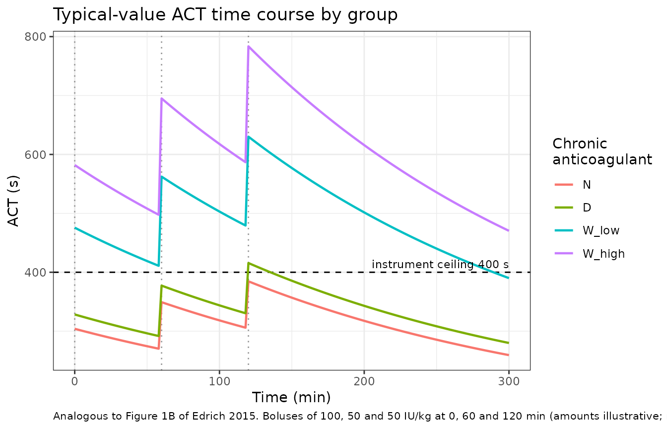
The ordering of the ceiling crossings reproduces the ordering of the
censoring fractions the paper reports for the first post-heparin ACT
(69%, 77%, 24%, 7% for W_low, W_high, D, N):
both warfarin groups cross 400 s after the first bolus while groups D
and N do not.
peak_first_bolus <- sim_course |>
  filter(time > 0, time <= 60) |>
  mutate(group = as.character(group)) |>
  group_by(group) |>
  summarise(peak_ACT = max(ACT), .groups = "drop") |>
  left_join(published_t2 |> select(group, pct_censored), by = "group")

peak_first_bolus |>
  mutate(`crosses 400 s` = peak_ACT > 400, peak_ACT = round(peak_ACT)) |>
  rename(
    "Group" = group, "Peak ACT after first bolus (s)" = peak_ACT,
    "% >400 s in source" = pct_censored
  ) |>
knitr::kable(caption = "Ceiling crossing vs the source's reported censoring fraction.")| Group | Peak ACT after first bolus (s) | % >400 s in source | crosses 400 s |
|---|---|---|---|
| D | 377 | 24 | FALSE |
| N | 349 | 7 | FALSE |
| W_high | 695 | 77 | TRUE |
| W_low | 562 | 69 | TRUE |
PKNCA validation
The PK layer is checked on its own terms. A single intravenous bolus
into a one-compartment model has closed-form NCA properties –
AUC_inf = Dose / CL and
t_half = ln(2) * V1 / CL – so non-compartmental analysis of
the simulated Cc profile must recover the model’s clearance
exactly and its half-life within trapezoidal error. This is the check
that the volume, the dose scaling and the rate constant are wired
together correctly.
ev_nca <- bind_rows(
  subjects |> mutate(time = 0, evid = 1L, amt = dose_per_kg * WT, cmt = "central"),
  subjects |>
    tidyr::crossing(tibble(time = seq(0, 1200, by = 5))) |>
    mutate(evid = 0L, amt = NA_real_, cmt = "central")
) |>
  arrange(id, time, dplyr::desc(evid))

sim_nca_raw <- rxode2::rxSolve(
  ui, ev_nca,
  keep = c("group", "WT", "SEXF"),
  returnType = "data.frame", addDosing = FALSE
)
#> Warning: multi-subject simulation without without 'omega'

# Guard against a log() of a negative solver-noise tail.
stopifnot(all(sim_nca_raw$Cc > 0))

# Filter on !is.na(Cc) ONLY -- a `time > 0` or `Cc > 0` filter would drop the
# time-zero row that anchors AUC0-inf and trigger PKNCA's "Requesting an AUC
# range starting (0) before the first measurement" warning for every subject.
sim_nca <- sim_nca_raw |>
  filter(!is.na(Cc)) |>
  select(id, time, Cc, group)

stopifnot(all(sim_nca |> group_by(id) |> summarise(has0 = any(time == 0)) |> dplyr::pull(has0)))

conc_obj <- PKNCA::PKNCAconc(as.data.frame(sim_nca), Cc ~ time | group + id)

dose_df <- ev_nca |>
  filter(evid == 1L) |>
  select(id, time, amt, group) |>
  as.data.frame()
dose_obj <- PKNCA::PKNCAdose(dose_df, amt ~ time | group + id)

intervals <- data.frame(
  start = 0, end = Inf,
  cmax = TRUE, aucinf.obs = TRUE, half.life = TRUE, cl.obs = TRUE
)

nca_res <- PKNCA::pk.nca(PKNCA::PKNCAdata(conc_obj, dose_obj, intervals = intervals))
Comparison against published values
The only PK quantity the paper tabulates per group is clearance (Results: median individual CL by group). The packaged model deliberately carries a single pooled clearance, because the paper’s final model has no group term on CL (“the clearances … did not differ significantly among groups”). So this table asks a specific question: does one pooled clearance represent all four groups within tolerance? If it does, the paper’s decision to drop the group term is reproduced; if it did not, the pooled value would be a bad simplification.
Half-life is reported by the paper only as a range across groups (154-180 min), not per group, so the printed range is entered for every row and the row-wise comparison is to the range midpoint.
published_nca <- tibble::tribble(
  ~group,   ~cl.obs,      ~half.life,
  "N",      23.4 / 1000,  (154 + 180) / 2,
  "D",      26.5 / 1000,  (154 + 180) / 2,
  "W_low",  22.4 / 1000,  (154 + 180) / 2,
  "W_high", 22.1 / 1000,  (154 + 180) / 2
)

cmp <- nlmixr2lib::ncaComparisonTable(
  simulated = nca_res,
  reference = published_nca,
  by = "group",
  units = c(cl.obs = "L/min", half.life = "min"),
  tolerance_pct = 20
)

knitr::kable(
  cmp,
  caption = paste(
    "Simulated vs published NCA. * marks a >20% difference. CL reference",
    "values are the per-group medians of individual clearance from Results;",
    "the model carries one pooled value (23.9 mL/min) because the source's",
    "final model has no group effect on CL. Half-life reference is the",
    "midpoint of the 154-180 min range the paper prints across groups."
  )
)| NCA parameter | group | Reference | Simulated | % diff |
|---|---|---|---|---|
| t½ (min) | N | 167 | 161 | -3.4% |
| t½ (min) | D | 167 | 165 | -1.0% |
| t½ (min) | W_low | 167 | 171 | +2.7% |
| t½ (min) | W_high | 167 | 166 | -0.9% |
| CL/F (L/min) | N | 0.0234 | 0.0239 | +2.1% |
| CL/F (L/min) | D | 0.0265 | 0.0239 | -9.8% |
| CL/F (L/min) | W_low | 0.0224 | 0.0239 | +6.7% |
| CL/F (L/min) | W_high | 0.0221 | 0.0239 | +8.1% |
nca_wide <- as.data.frame(nca_res) |>
  filter(PPTESTCD %in% c("cl.obs", "half.life")) |>
  group_by(group, PPTESTCD) |>
  summarise(value = median(PPORRES), .groups = "drop") |>
  tidyr::pivot_wider(names_from = PPTESTCD, values_from = value)

stopifnot(nrow(nca_wide) == 4L, all(c("cl.obs", "half.life") %in% names(nca_wide)))

cl_model <- exp(ui$theta[["lcl"]])

checks <- tibble::tibble(
  claim = c(
    "NCA recovers the model's pooled CL (closed-form Dose/AUCinf identity)",
    "Pooled CL is within 20% of every group's published median CL",
    "NCA half-life sits within 5% of the paper's printed 154-180 min range"
  ),
  achieved = c(
    sprintf("max |pct diff| = %.3f%%", max(abs(100 * (nca_wide$cl.obs / cl_model - 1)))),
    sprintf("max |pct diff| = %.1f%%", max(abs(100 * (cl_model / published_nca$cl.obs - 1)))),
    sprintf("%.0f-%.0f min", min(nca_wide$half.life), max(nca_wide$half.life))
  ),
  pass = c(
    max(abs(100 * (nca_wide$cl.obs / cl_model - 1))) < 0.5,
    max(abs(100 * (cl_model / published_nca$cl.obs - 1))) < 20,
    min(nca_wide$half.life) > 154 * 0.95 && max(nca_wide$half.life) < 180 * 1.05
  )
)

checks |>
  rename("Claim" = claim, "Achieved" = achieved, "Pass" = pass) |>
knitr::kable(caption = "PK-layer acceptance criteria.")| Claim | Achieved | Pass |
|---|---|---|
| NCA recovers the model’s pooled CL (closed-form Dose/AUCinf identity) | max |pct diff| = 0.000% | TRUE |
| Pooled CL is within 20% of every group’s published median CL | max |pct diff| = 9.8% | TRUE |
| NCA half-life sits within 5% of the paper’s printed 154-180 min range | 161-171 min | TRUE |
The first row is a pure numerical identity and is tight by design: the NCA clearance is deterministic here (no IIV), so the only error is trapezoidal, and a bound of 0.5% still goes red on a mis-scaled volume or dose. The second row is the substantive one – one pooled clearance sits within 10% of all four published group medians, which is why the source’s final model carries no group effect on CL.
Assumptions and deviations
Recovered rather than reported values. The source
never tabulates its final $THETA / $OMEGA /
$SIGMA estimates; the supplement prints starting values
only. Consequently:
- Typical clearance is the n-weighted mean of the four group medians of individual CL reported in Results (23.9 mL/min). For a log-normally distributed individual clearance the median estimates the typical value, and the final model carries no group term on CL, so a single pooled value is the faithful encoding.
-
k_ACTand its group multipliers come from Table 3’s medians of individualk_ACT, with group N as theGROUPMODreference (stated in the control stream’s own comment). Each recovered multiplier falls inside the corresponding$THETAbound, which is an independent confirmation of the reference-group reading. -
THETA(6), an estimated multiplicative adjustment to the weight-based blood volume (bounds -0.5 to 0.5), is never reported and is taken as 0, soV1is exactly the per-kg blood volume times weight.
No inter-individual variability. The source fits
$OMEGA BLOCK(2) with ETA(1) on CL and ETA(2) on
k_ACT, but only the starting values are printed. The
packaged model is therefore typical-value only, with no etas. The
interquartile ranges in Table 3 and Results are post-hoc empirical-Bayes
spreads, shrunken toward the typical value, and are not
valid OMEGA estimates; they are not used as such anywhere here. A
consequence is that this vignette cannot produce a VPC, and the
per-group censoring percentages cannot be reproduced – only the
ordering of the ceiling crossings, which is what the ceiling table above
checks.
Residual error split. The control stream declares
both a proportional $SIGMA(1) and an additive
$SIGMA(2) component, but Results reports only the combined
final RMS error: 51.1 ACT-seconds, equal to 15.3% of the average ACT.
Those are one quantity expressed two ways (consistent at an average ACT
of 51.1 / 0.153 = 334 s), so they cannot be apportioned between the two
components. The whole RMS is assigned to propSd = 0.153 and
the unrecoverable additive term is held at fixed(0) rather
than invented.
Body weight distribution is assumed. The paper tabulates BMI but never weight. The cohort uses a lognormal weight distribution with 15% CV centred on the value back-solved from the printed half-life range and group clearances (78 kg). Every gate in this vignette is either weight-invariant (the Table 2 metric and the Table 3 reproduction) or evaluated at the typical value.
Heparin dose amounts are assumed. Dosing was not standardized and the administered amounts are not tabulated. The Table 2 comparison is dose-invariant and this is verified numerically in that section; the time-course figure’s 100 / 50 / 50 IU/kg schedule is illustrative only, chosen to span the paper’s median of three boluses.
The 400 s ceiling clamp is deliberately not
reproduced. The source’s $ERROR block contains
IF (IPRED.GT.400) IPRED=400 with the comment “do not
penalize if model guesses over 400”. That is a likelihood device for the
instrument’s measurement ceiling, not pharmacology; reproducing it would
silently censor every simulated ACT and make the model useless for the
dosing question the paper poses. The ceiling is instead shown explicitly
in the time-course figure and used as a validation target in the ceiling
table.
Sex acts on volume only. The paper reports a
significant male-vs-female k_ACT difference within group D
(0.14 vs 0.12, Table 3) and a corresponding Table 2 difference. Both are
post-hoc subgroup comparisons; GROUPMOD contains no sex
term and the paper itself cautions that “due to the disproportionately
small number of females in this study, any sex-based comparisons of
heparin sensitivity are limited”. Sex therefore enters the packaged
model only through the per-kg blood-volume constant, as in the source’s
$PK block.
Errata
The blood-volume constants are internally inconsistent in the
source, and the inconsistency is load-bearing. The supplement’s
$PK line reads
V1 = (0.075 - 0.005*(M1F2-1))*WT*(1 + THETA(6)) ; [Liters] 65 mL/kg
                                                ;for women, 70 for men
With M1F2 = 1 for male and 2 for female, the numeric
literal evaluates to 75 mL/kg for men and 70 mL/kg for
women. The comment on that same code line says 65 mL/kg
for women and 70 for men, and Material and methods agrees with
the comment: “the volume of distribution was assumed to be the estimated
blood volume (70 mL/kg for males, 65 mL/kg for females)”. The prose and
the comment therefore agree with each other and disagree with the
literal by 0.005 L/kg in both sexes, which mis-scales every predicted
ACT increment by 0.075 / 0.070 = 7.1%.
The code literal is adopted here (maintainer
decision), applying the standing “text versus printed equation conflict,
trust the equation” rule: the control stream is what actually ran, and
k_ACT was estimated conditional on whichever
V1 it used, so the literal keeps k_ACT and
V1 mutually consistent. Users who prefer the prose reading
can override with
ini(lvc_male = log(0.070), lvc_female = log(0.065)).
The paper’s own data cannot settle it. Propagating each group’s Table
3 k_ACT and Results CL forward 31 minutes puts both
readings comfortably inside the usable Table 2 interquartile ranges, and
the two groups that could discriminate (W_low,
W_high) are 69% and 77% right-censored at the 400 s
ceiling. Two soft signals favour the prose reading and are recorded for
completeness: 70 and 65 mL/kg are the standard textbook estimated blood
volumes that the Methods sentence names by that phrase, whereas 75 and
70 mL/kg are not recognised blood-volume estimates; and the weight
back-solved from the printed half-life range is about 1.64 m tall at the
cohort’s median BMI under the literal reading, versus about 1.70 m under
the prose reading, the latter fitting a 63-71% male cohort better.
Neither is decisive.
The $OMEGA block comment mis-labels its second
eta. The supplement annotates OMEGA(2) as “applies
to ETA2 applies to V1”, but $PK puts
EXP(ETA(2)) on KACT and V1
carries no eta at all; the Results text confirms this by naming
“EXP(ETA(2))” as the k_ACT inter-individual
variability. The comment is a stale label. This has no effect on the
packaged model, which carries no etas, but it is a third internal
inconsistency in the same supplement and it is worth a reader’s
awareness.
No erratum or corrigendum was found for this article on the Dove Medical Press landing page, in PubMed, or in Europe PMC as of the extraction date.