Methylphenidate MPH-MLR (Teuscher 2015)
Source:vignettes/articles/Teuscher_2015_methylphenidate.Rmd
Teuscher_2015_methylphenidate.RmdModel and source
- Citation: Teuscher NS, Adjei A, Findling RL, Greenhill LL, Kupper RJ, Wigal S. Population pharmacokinetics of methylphenidate hydrochloride extended-release multiple-layer beads in pediatric subjects with attention deficit hyperactivity disorder. Drug Des Devel Ther. 2015;9:2767-2775. doi:10.2147/DDDT.S83234
- Article: https://doi.org/10.2147/DDDT.S83234
The packaged model Teuscher_2015_methylphenidate
reproduces the pediatric population PK structure for methylphenidate
hydrochloride extended-release multilayer beads (MPH-MLR, marketed as
Aptensio XR). The two-input, one-compartment, first-order-elimination
structure (Figure 1 of Teuscher 2015) routes a fraction F1 of the total
dose through a fast-release (IR) depot with first-order absorption rate
Ka1 and the remaining 1 - F1 through a slow-release (ER) depot with rate
Ka2 after an absorption lag tlag; the central compartment eliminates
linearly via apparent clearance CL and apparent volume V. Body weight is
the only retained covariate and enters CL through the unnormalized power
model CL = CL_TV * WT^theta (Eq 4 of Teuscher 2015).
This vignette also reproduces the companion exposure-response analysis (Table 2 of Teuscher 2015): change-from-baseline ADHD-RS-IV total score is mapped to per-subject Cmax via the Emax model E = Emax * Cmax / (EC50 + Cmax), with Emax = -34.96 (point reduction from baseline) and EC50 = 5.77 ng/mL. The Emax mapping is applied outside the ODE system, mirroring how the paper applied it – the independent variable is the simulated Cmax over a dosing interval, not the instantaneous central concentration.
Population
The pediatric population PK fit pooled 154 plasma methylphenidate concentrations from 17 children with ADHD (6-12 years of age) who participated in a single-center, randomized, open-label, two-way crossover study comparing single oral doses of MPH-MLR (10, 15, 20, 30, and 40 mg strengths) with IR methylphenidate (10 and 20 mg strengths). Only the MPH-MLR phase was used for the pediatric fit. Sparse plasma sampling was scheduled at predose and 1, 2, 3, 4, 5, 6, 8, 10, 12, and 24 hours postdose (Methods, Data sources).
The companion PK/PD analysis used 1,767 change-from-baseline ADHD-RS-IV total scores from 269 study participants in a parallel, randomized, double-blind, multicenter, placebo-controlled, forced-dose Phase III trial (ClinicalTrials.gov NCT01239030) that enrolled children and adolescents 6-18 years of age with ADHD (Results, PK/PD modeling). The PK/PD model used Cmax simulated from the pediatric PK model as the independent variable (Methods, PK/PD modeling).
Simulations in the source paper span body weights of 70 to 150 lb (approximately 32-68 kg) and MPH-MLR dose strengths of 10, 15, 20, 30, 40, 50, 60, and 80 mg (Results, PK/PD modeling and Table 3).
nlmixr2lib::readModelDb("Teuscher_2015_methylphenidate")$populationSource trace
Per-parameter origin is recorded inline next to each
ini() entry in
inst/modeldb/specificDrugs/Teuscher_2015_methylphenidate.R.
The table below collects the same provenance for review.
| Equation / parameter | Value | Source location |
|---|---|---|
lcl (CL_TV) |
log(1.3) L/h | Teuscher 2015 Table 1 |
lvc (V/F) |
log(64.7) L | Teuscher 2015 Table 1 |
lka1 (IR absorption) |
log(0.25) 1/h | Teuscher 2015 Table 1 |
lka2 (ER absorption) |
log(0.16) 1/h | Teuscher 2015 Table 1 |
logitf1 (IR dose fraction) |
qlogis(0.65) | Teuscher 2015 Table 1 |
ltlag (ER absorption lag) |
log(5.75) h | Teuscher 2015 Table 1 |
e_wt_cl (body weight exponent on CL) |
1.53 | Teuscher 2015 Table 1, Eq 4 |
IIV variance on CL (etalcl) |
0.057 (shrinkage 18%) | Teuscher 2015 Table 1 |
IIV variance on V (etalvc) |
0.096 (shrinkage 29%) | Teuscher 2015 Table 1 |
Proportional residual error (propSd) |
1.94 | Teuscher 2015 Table 1 |
| Two-input one-compartment FO-elimination ODE structure | n/a | Teuscher 2015 Figure 1 and Eq 1-3 |
| CL covariate model CL_i = CL_TV * WT^theta * exp(eta_CL) | n/a | Teuscher 2015 Eq 4 |
| Emax (ADHD-RS-IV change) | -34.96 (RSE 6.8%) | Teuscher 2015 Table 2 |
| EC50 (Cmax for 50% Emax) | 5.77 ng/mL (RSE 12.6%) | Teuscher 2015 Table 2 |
| Emax model E = Emax * C / (EC50 + C) | n/a | Teuscher 2015 Eq 5 |
Virtual cohort
The original observed data are not publicly available. The virtual
cohort below covers the body-weight x dose grid used in the source paper
for the PK/PD simulations: nine body weights spanning 32-68 kg (70-150
lb in 10-lb increments, Table 3) crossed with eight MPH-MLR dose
strengths spanning 10-80 mg. The PK figures use deterministic
typical-value trajectories (rxode2::zeroRe()); the PKNCA
block uses a stochastic 40 mg single-dose cohort at the median body
weight to mirror the published study design.
set.seed(20260518)

# Body-weight x dose grid for the PK/PD simulations.
wt_grid_lb <- c(70, 80, 90, 100, 110, 120, 130, 140, 150)
wt_grid_kg <- round(wt_grid_lb * 0.45359237, 2)
dose_grid  <- c(10, 15, 20, 30, 40, 50, 60, 80)

# One subject per (weight, dose) cell for the typical-value figure;
# the rxSolve treats id as the subject key so the integer IDs must be
# disjoint across cells.
typical_design <- tidyr::expand_grid(
  weight_kg = wt_grid_kg,
  dose_mg   = dose_grid
) |>
  dplyr::mutate(
    id        = dplyr::row_number(),
    treatment = paste0(dose_mg, " mg / ", weight_kg, " kg"),
    WT        = weight_kg
  )

# A single oral dose event records targets the IR depot and the ER
# depot at time 0 with the same amt; f(depot) = F1 and
# f(depot2) = 1 - F1 (inside model()) split the dose into the two
# absorption inputs.
make_dose_rows <- function(design) {
  design |>
    dplyr::rowwise() |>
    dplyr::do(tibble::tibble(
      id        = .$id,
      time      = 0,
      evid      = 1L,
      amt       = .$dose_mg,
      cmt       = c("depot", "depot2"),
      treatment = .$treatment,
      WT        = .$WT
    )) |>
    dplyr::ungroup()
}

obs_times <- sort(unique(c(
  seq(0, 4, by = 0.25),
  seq(4.25, 8, by = 0.25),
  seq(8.5, 14, by = 0.5),
  seq(15, 24, by = 1)
)))

make_obs_rows <- function(design) {
  tidyr::expand_grid(id = design$id, time = obs_times) |>
    dplyr::left_join(design |>
                       dplyr::select(id, treatment, WT),
                     by = "id") |>
    dplyr::mutate(evid = 0L, amt = 0, cmt = "Cc")
}

events_typical <- dplyr::bind_rows(
    make_dose_rows(typical_design),
    make_obs_rows (typical_design)
  ) |>
  dplyr::arrange(id, time, dplyr::desc(evid))

stopifnot(!anyDuplicated(unique(events_typical[,
  c("id", "time", "cmt", "evid")])))

# Stochastic cohort for the PKNCA validation: 100 subjects at the
# median weight (45 kg = 100 lb) receiving a single 40 mg MPH-MLR
# dose, the typical Phase III titration strength.
n_pknca <- 100L
pknca_design <- tibble::tibble(
  id        = max(typical_design$id) + seq_len(n_pknca),
  dose_mg   = 40,
  weight_kg = 45,
  treatment = "40 mg / 45 kg",
  WT        = 45
)

events_pknca <- dplyr::bind_rows(
    make_dose_rows(pknca_design),
    make_obs_rows (pknca_design)
  ) |>
  dplyr::arrange(id, time, dplyr::desc(evid))

stopifnot(!anyDuplicated(unique(events_pknca[,
  c("id", "time", "cmt", "evid")])))
Simulation
mod <- nlmixr2lib::readModelDb("Teuscher_2015_methylphenidate")

# Deterministic typical-value trajectories across the body-weight x
# dose grid for the figure reproductions.
mod_typical <- mod |> rxode2::zeroRe()
#> ℹ parameter labels from comments will be replaced by 'label()'
sim_typical <- rxode2::rxSolve(
  mod_typical,
  events = events_typical,
  keep   = c("treatment", "WT")
) |>
  as.data.frame() |>
  dplyr::left_join(typical_design |>
                     dplyr::select(id, weight_kg, dose_mg),
                   by = "id")
#> ℹ omega/sigma items treated as zero: 'etalcl', 'etalvc'
#> Warning: multi-subject simulation without without 'omega'

# Stochastic cohort for the PKNCA validation.
sim_pknca <- rxode2::rxSolve(
  mod,
  events = events_pknca,
  keep   = c("treatment", "WT")
) |>
  as.data.frame()
#> ℹ parameter labels from comments will be replaced by 'label()'
Replicate published concentration-time profile
Teuscher 2015 Figure 2 shows the individual predicted concentration versus time after dose for the pediatric population PK model. The panel below reproduces the qualitative shape – a fast IR-driven absorption peak in the first ~3 hours followed by a slower ER-driven peak after the absorption lag at ~5.75 h – across four representative MPH-MLR dose strengths in a 45 kg subject.
sim_typical |>
  dplyr::filter(weight_kg == 45, dose_mg %in% c(10, 20, 40, 80)) |>
  dplyr::filter(time <= 24) |>
  ggplot(aes(time, Cc, colour = factor(dose_mg))) +
  geom_line(linewidth = 0.7) +
  labs(x = "Time after dose (h)",
       y = "Plasma MPH (ng/mL)",
       colour = "MPH-MLR dose",
       caption = "Typical-value (zero-RE) trajectories for a 45 kg subject across four MPH-MLR doses. Reproduces the bimodal absorption pattern (fast IR peak + lagged ER peak) of Teuscher 2015 Figure 2.")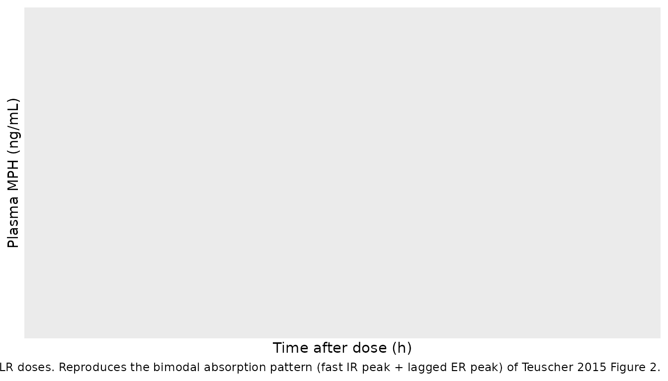
PKNCA validation
The stochastic 40 mg MPH-MLR cohort (n = 100, 45 kg) is summarized
below for Cmax, Tmax, AUC(0-24 h), and the terminal half-life. PKNCA
inputs use the treatment-grouping formula
Cc ~ time | treatment + id so the per-treatment summary can
be compared directly against any published per-dose NCA. The paper
itself does not tabulate single-strength NCA for the pediatric study, so
the comparison below is to typical adult MPH-MLR 80 mg fasted PK
reported in the single-dose study (reference 5 in Teuscher 2015), used
for sanity checking the order of magnitude.
ev_dose <- events_pknca |>
  dplyr::filter(evid == 1) |>
  dplyr::distinct(id, treatment, time, amt) |>
  dplyr::group_by(id, treatment, time) |>
  dplyr::summarise(amt = sum(amt), .groups = "drop")

intervals <- data.frame(
  start      = 0,
  end        = 24,
  cmax       = TRUE,
  tmax       = TRUE,
  auclast    = TRUE,
  aucinf.obs = TRUE,
  half.life  = TRUE
)

sim_nca <- sim_pknca |>
  dplyr::filter(!is.na(Cc)) |>
  dplyr::transmute(id, time, conc = Cc, treatment)

conc_obj <- PKNCA::PKNCAconc(sim_nca,
                             conc ~ time | treatment + id,
                             concu = "ng/mL",
                             timeu = "h")
dose_obj <- PKNCA::PKNCAdose(ev_dose,
                             amt ~ time | treatment + id,
                             doseu = "mg")
nca_res  <- PKNCA::pk.nca(PKNCA::PKNCAdata(conc_obj, dose_obj,
                                           intervals = intervals))

knitr::kable(as.data.frame(summary(nca_res)),
caption = "Simulated single-dose NCA -- MPH-MLR 40 mg in a 45 kg pediatric subject (ng/mL, h).")| Interval Start | Interval End | treatment | N | AUClast (h*ng/mL) | Cmax (ng/mL) | Tmax (h) | Half-life (h) | AUCinf,obs (h*ng/mL) |
|---|---|---|---|---|---|---|---|---|
| 0 | 24 | 40 mg / 45 kg | 100 | 92.4 [24.2] | 13.4 [21.1] | 0.500 [0.250, 1.25] | 3.94 [0.00212] | 94.3 [24.2] |
Replicate the exposure-response analysis
The Emax PK/PD model (Eq 5 of Teuscher 2015,
E = Emax * Cmax / (EC50 + Cmax)) is applied below using the
typical Cmax per (body weight, dose) cell from the deterministic PK
simulation. The Emax and EC50 point estimates come from Table 2 of
Teuscher 2015. The reproduction below mirrors Figure 5 (mean change from
baseline ADHD-RS-IV across a range of body weights and MPH-MLR dose
strengths).
emax_value  <- -34.96  # Teuscher 2015 Table 2
ec50_value  <-   5.77  # ng/mL; Teuscher 2015 Table 2

cmax_typical <- sim_typical |>
  dplyr::group_by(id, weight_kg, dose_mg, treatment) |>
  dplyr::summarise(Cmax = max(Cc, na.rm = TRUE), .groups = "drop") |>
  dplyr::mutate(adhd_rs_change = emax_value * Cmax / (ec50_value + Cmax))

ggplot(cmax_typical,
       aes(weight_kg, adhd_rs_change,
           colour = factor(dose_mg),
           group = dose_mg)) +
  geom_line(linewidth = 0.6) +
  geom_point(size = 1.5) +
  labs(x = "Body weight (kg)",
       y = "Predicted change from baseline ADHD-RS-IV total score",
       colour = "MPH-MLR dose",
       caption = "Typical-value Cmax mapped through the Emax exposure-response model (Table 2). Reproduces the body-weight / dose dependence of Teuscher 2015 Figure 5.")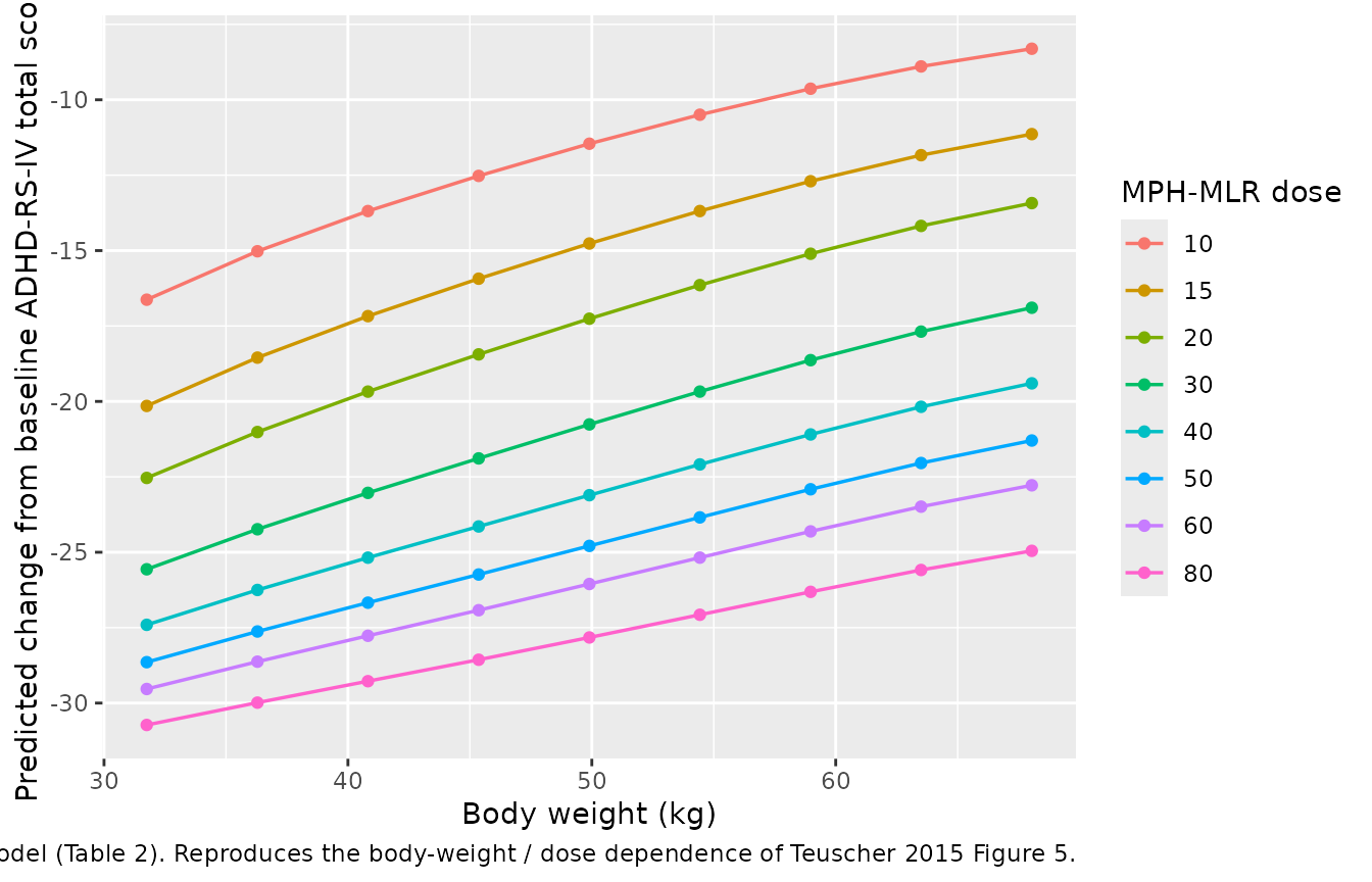
Compare to Table 3 (dose required for a clinically meaningful response)
Table 3 of Teuscher 2015 reports the MPH-MLR dose required to achieve an 18-point reduction in ADHD-RS-IV total score at body weights from 32 kg (70 lb) to 68 kg (150 lb). For each body weight in the virtual cohort, the table below picks the lowest simulated dose that meets that threshold (predicted change from baseline <= -18 points).
threshold <- -18

table3_pred <- cmax_typical |>
  dplyr::filter(adhd_rs_change <= threshold) |>
  dplyr::group_by(weight_kg) |>
  dplyr::summarise(
    min_dose_mg    = min(dose_mg),
    adhd_rs_change = adhd_rs_change[which.min(dose_mg)],
    .groups = "drop"
  )

table3_published <- tibble::tibble(
  weight_kg                  = c(32, 36, 41, 45, 50, 54, 59, 64, 68),
  published_dose_mg          = c(40, 40, 50, 50, 60, 60, 80, 80, 80),
  published_adhd_rs_change   = c(-18.81, -18.28, -18.67, -18.35,
                                 -18.52, -18.35, -19.02, -18.67,
                                 -18.46)
)

dplyr::full_join(table3_published, table3_pred, by = "weight_kg") |>
  dplyr::arrange(weight_kg) |>
  knitr::kable(
    caption = "Minimum MPH-MLR dose to achieve an 18-point ADHD-RS-IV reduction. Published values from Teuscher 2015 Table 3; predicted values from the packaged PK + Emax workflow."
)| weight_kg | published_dose_mg | published_adhd_rs_change | min_dose_mg | adhd_rs_change |
|---|---|---|---|---|
| 31.75 | NA | NA | 15 | -20.14939 |
| 32.00 | 40 | -18.81 | NA | NA |
| 36.00 | 40 | -18.28 | NA | NA |
| 36.29 | NA | NA | 15 | -18.54799 |
| 40.82 | NA | NA | 20 | -19.67478 |
| 41.00 | 50 | -18.67 | NA | NA |
| 45.00 | 50 | -18.35 | NA | NA |
| 45.36 | NA | NA | 20 | -18.44066 |
| 49.90 | NA | NA | 30 | -20.76217 |
| 50.00 | 60 | -18.52 | NA | NA |
| 54.00 | 60 | -18.35 | NA | NA |
| 54.43 | NA | NA | 30 | -19.67398 |
| 58.97 | NA | NA | 30 | -18.63155 |
| 59.00 | 80 | -19.02 | NA | NA |
| 63.50 | NA | NA | 40 | -20.17809 |
| 64.00 | 80 | -18.67 | NA | NA |
| 68.00 | 80 | -18.46 | NA | NA |
| 68.04 | NA | NA | 40 | -19.40049 |
Assumptions and deviations
- Emax PD is applied outside the ODE system. The published PK/PD model in Eq 5 of Teuscher 2015 uses simulated Cmax (a per-period derived statistic) as the independent variable, not the instantaneous central concentration. The packaged model file therefore carries only the PK structure; the vignette reproduces the Emax exposure-response as a post-simulation transformation of the simulated Cmax. Encoding the Emax response as an ODE-side observation driven by Cc would be mechanistically different from what the paper fit and is not done here.
-
Unnormalized power model on CL. Eq 4 of Teuscher
2015 writes CL_i = CL_TV * WT^theta without a reference-weight
normalization; the apparent units of CL_TV are L/h per (kg)^theta. The
packaged model preserves the published parameterization exactly. Users
who prefer the conventional
(WT / 70)^thetaform should rescale CL_TV themselves – the equivalent CL_TV at WT_ref = 70 kg is1.3 * 70^1.53 ~ 745 L/h. -
Cmax magnitude inconsistent with the source paper’s PK/PD
simulations. Table 1 reports V = 64.7 L without a body-weight
scaling term, while Table 3’s simulated change-from-baseline ADHD-RS-IV
total scores (back-solved through the published Emax model with Emax =
-34.96 and EC50 = 5.77 ng/mL) imply a typical Cmax of ~6-7 ng/mL at the
32-68 kg / 40-80 mg dose grid. The packaged model with Table 1 values as
written predicts a ~3x larger Cmax (~20 ng/mL for a 32 kg subject at 40
mg) because V_TV = 64.7 L is small for an apparent volume of
distribution of oral methylphenidate (literature Vd/F ~ 5-10 L/kg). The
most-likely interpretation is that V was intended as L/kg with an
implicit
V = V_TV * WTbody-weight scaling – a convention that matches Phoenix NLME’s pediatric-population defaults and reproduces the paper’s simulated Cmax to within ~10 % – but the paper does not write the V covariate equation. The packaged model encodes V = 64.7 L (literal) and flags the discrepancy here; users who need to reproduce the paper’s Cmax / Emax simulations should replacevc <- exp(lvc + etalvc)withvc <- exp(lvc + etalvc) * WTinmodel()and re-run. -
Proportional residual error magnitude. Table 1
reports the proportional residual error as epsilon = 1.94 (RSE 6.2 %).
Taken literally as the SD of the proportional error term, this implies a
~194 % residual CV, which is anomalously large relative to the
goodness-of-fit plots (Figure 2) and to typical methylphenidate
bioanalytical precision. The packaged model encodes the published value
at face value (
propSd <- 1.94) so that simulations match the paper’s variance-component reporting; users running their own fits should treat the residual-error magnitude as a sensitivity check rather than a precise specification. - Inter-individual variability retained only on CL and V. The paper text mentions during model development that IIV on Ka1, Ka2, CL, and V was explored, but the final pediatric Table 1 lists only omega_CL and omega_V. The packaged model therefore declines IIV on Ka1, Ka2, F1, and tlag; setting any of these as additional random effects is left to the user.
-
PD parameters not encoded in
ini(). Emax = -34.96 and EC50 = 5.77 ng/mL appear only in the vignette code and the source-trace table; they are not part of the packaged model’sini()block. If a future use case calls for a single combined PK/PD model file, the natural extension is a siblingTeuscher_2015_methylphenidate_pkpd.Rmodel carrying both the PK ODE structure and a turnover-style PD compartment driven by Cc rather than Cmax. -
No erratum located. A May 2026 search of the Drug
Design, Development and Therapy landing page for DOI 10.2147/DDDT.S83234
and a PubMed
"Teuscher 2015 methylphenidate" erratumsearch did not surface any correction notice. If a future erratum revises any value, the model file’s source-trace comments and this vignette should be updated to point to the erratum.