Paroxetine cumulative exposure and depression-severity response (Shigetome 2025)
Source:vignettes/articles/Shigetome_2025_paroxetine.Rmd
Shigetome_2025_paroxetine.RmdModels and source
Shigetome 2025 reports two models fitted in two separate NONMEM runs on two different cohorts, so the paper contributes two model files:
pk_ui <- rxode2::rxode(readModelDb("Shigetome_2025_paroxetine"))
#> ℹ parameter labels from comments will be replaced by 'label()'
pd_ui <- rxode2::rxode(readModelDb("Shigetome_2025_paroxetine_madrs"))
#> ℹ parameter labels from comments will be replaced by 'label()'- Citation: Shigetome K, Egashira T, Tomita T, Higa N, Iwashita K, Morita K, Nishimura M, Kaneko T, Maeda H, Yamada KD, Kajiwara-Morita A, Oniki K, Yasui-Furukori N, Saruwatari J. Effect of Cumulative Exposure on the Efficacy of Paroxetine: A Population Pharmacokinetic-Pharmacodynamic and Machine Learning Analyses. CPT Pharmacometrics Syst Pharmacol. 2025 Jun;14(6):1119-1127. doi:10.1002/psp4.70032.
- Article: https://doi.org/10.1002/psp4.70032
- Supplementary Information (Tables S1-S5, Figures S1-S6, Texts S1-S4 including both NONMEM control streams): https://europepmc.org/article/PMC/PMC12167921
Shigetome_2025_paroxetine – population
PK, 329 steady-state concentrations from 179 patients.
One-compartment population PK model for paroxetine in 179 Japanese adults with major depressive disorder treated at Hirosaki University Hospital or Dokkyo Medical University, fitted to 329 steady-state plasma concentrations (therapeutic drug monitoring). Neither an absorption process nor saturable metabolism improved the fit, so oral doses enter the central compartment directly and CL/F and Vd/F are apparent oral parameters. Apparent clearance carries power covariate effects of age (exponent -0.536, higher age = lower CL) and total body weight (exponent 0.563), both normalized to the study means (41.5 years, 58.6 kg); CYP2D6 genotype was tested in three classifications and had no significant effect. Vd/F was fixed at 1010 L (mean body weight 58.6 kg times a literature Vd/F of 17.2 L/kg) because sparse trough sampling could not support its estimation. Exponential inter-individual variability on CL and a proportional residual error.
Shigetome_2025_paroxetine_madrs –
population PK-PD, MADRS time course in the 50-patient subset with serial
depression ratings.
Population PK-PD model for the time course of depression-severity improvement under paroxetine in 50 Japanese adults with major depressive disorder, fitted to Montgomery-Asberg Depression Rating Scale (MADRS) scores at baseline and weeks 1, 2, 4 and 6. The endpoint madrsenh is the paper’s enhancement rate, the percentage reduction in MADRS from baseline, described by an Emax model in treatment duration: madrsenh = Emax * Time / (ET50 + Time). Cumulative paroxetine exposure over the first week of treatment (AUC_PAROX, predicted from the companion popPK model Shigetome_2025_paroxetine) enters Emax through the power term -(AUC_PAROX / 2610.43)^-8.56, so higher first-week exposure raises the attainable improvement; the MADRS score at week 1 (SCORE_MADRS) enters ET50 through +(SCORE_MADRS / 28.64)^2.38, so less severe week-1 depression brings the improvement forward. There is no PK compartment and no dosing event in this model: drug exposure is carried entirely by the AUC_PAROX covariate, and the independent variable is treatment duration in weeks. Proportional inter-individual variability on both Emax and ET50, additive residual error.
The paper also develops six machine-learning classifiers (logistic regression, decision tree, k-nearest neighbour, support vector machine, random forest, multi-layer perceptron) predicting week-6 remission, with SHAP attribution. Those are classifiers rather than pharmacometric models and are not part of this extraction; the two nonlinear mixed-effects models above are.
Population
The PK cohort is 179 Japanese adults with DSM-IV major depressive disorder treated at Hirosaki University Hospital or Dokkyo Medical University School of Medicine, all antidepressant-naive at paroxetine initiation, with normal renal and hepatic function and no interacting co-medication (Shigetome 2025 Table 1). Age was 41.5 years (SD 14.2, range 16-80), body weight 58.6 kg (SD 10.5, range 40-85) and 40.8% were male. Paroxetine was started at 10-20 mg/day and titrated by 10 mg/day weekly to the maximum tolerated dose, giving a mean of 22.3 mg/day (SD 11.1, range 10-40). Sampling was sparse therapeutic drug monitoring: 1.8 samples per patient (range 1-5), all at steady state after at least 9 days on a stable dose, giving observed plasma concentrations of 51.9 ng/mL (SD 49.0, range 2.6-286.5). CYP2D6 genotyping found 121 intermediate metabolizers (67.6%) and 58 extensive metabolizers (32.4%); there were no poor metabolizers, which the authors attribute to the low frequency of null alleles in East Asians.
The PK-PD cohort is the 50-patient subset who also had MADRS ratings at baseline and weeks 1, 2, 4 and 6 plus a pre-treatment Temperament and Character Inventory (Table 2). That subset is slightly older (46.6 years, SD 13.7), slightly lighter (56.3 kg, SD 10.4) and received higher doses (32.2 mg/day, SD 11.0). Baseline MADRS was 39.6 (SD 9.7) falling to 13.7 (SD 12.9) by week 6; 26 of the 50 reached remission (MADRS < 10 at week 6).
The same information is available programmatically:
str(readModelDb("Shigetome_2025_paroxetine")()$population, max.level = 1)
#> List of 15
#>  $ species       : chr "human"
#>  $ n_subjects    : int 179
#>  $ n_studies     : int 1
#>  $ n_observations: int 329
#>  $ age_range     : chr "16-80 years"
#>  $ age_mean      : chr "41.5 years (SD 14.2)"
#>  $ weight_range  : chr "40-85 kg"
#>  $ weight_mean   : chr "58.6 kg (SD 10.5)"
#>  $ sex_female_pct: num 59.2
#>  $ race_ethnicity: Named num 100
#>   ..- attr(*, "names")= chr "Asian"
#>  $ disease_state : chr "major depressive disorder (DSM-IV), antidepressant-naive at paroxetine initiation, normal renal and hepatic fun"| __truncated__
#>  $ dose_range    : chr "10-40 mg/day orally (mean 22.3 mg/day, SD 11.1); initial dose 10-20 mg/day then weekly increases of 10 mg/day t"| __truncated__
#>  $ regions       : chr "Japan (Hirosaki University Hospital and Dokkyo Medical University School of Medicine)"
#>  $ genotype      : chr "CYP2D6 intermediate metabolizers 121 (67.6%), extensive metabolizers 58 (32.4%), poor metabolizers 0 (0%); *1/*"| __truncated__
#>  $ notes         : chr "Retrospective therapeutic-drug-monitoring cohort; 1.8 samples per patient on average (range 1-5), all drawn at "| __truncated__
Source trace
Every ini() entry carries an in-file comment naming its
source location. The tables below collect them. Point estimates for both
models live only in the Supporting Information (Tables S2 and S4); the
main text prints the final model equations but no parameter table.
Population PK (Shigetome_2025_paroxetine)
| Equation / parameter | Value | Source location |
|---|---|---|
CL/F = 23.6 * (AGE/41.5)^-0.536 * (WT/58.6)^0.563 |
– | Results 3.2, printed final popPK model equation |
Vd/F = 1010 L |
– | Methods 2.3 and Results 3.2; NONMEM $THETA 1010 FIX
(Text S2) |
| One compartment, no absorption process | – | Methods 2.3; NONMEM $SUBROUTINES ADVAN1 TRANS2 (Text
S2) |
Cc = 1000 * central / vc (mg, L -> ng/mL) |
– | NONMEM $PK S1 = V / 1000 (Text S2) |
lcl (CL/F) |
23.6 L/h | Table S2 (RSE 4.75%, bootstrap 95% CI 21.4-25.9) |
lvc (Vd/F, fixed) |
1010 L | Table S2 (fixed; 58.6 kg x 17.2 L/kg from the cited literature) |
e_age_cl |
-0.536 | Table S2 (RSE 25.4%, bootstrap 95% CI -0.790 to -0.270) |
e_wt_cl |
0.563 | Table S2 (RSE 48.9%, bootstrap 95% CI -0.01 to 1.19) |
etalcl (variance) |
0.307 | Table S2 (RSE 15.7%, shrinkage 7.83%, bootstrap 95% CI 0.197-0.392) |
propSd = sqrt(0.155) |
0.394 | Table S2 proportional error 0.155 (RSE 10.8%, shrinkage 19.3%) |
Population PK-PD (Shigetome_2025_paroxetine_madrs)
| Equation / parameter | Value | Source location |
|---|---|---|
EFF = Emax * Time / (ET50 + Time) |
– | Methods 2.3 printed Emax equation; NONMEM $PRED (Text
S3) |
Emax = 90.9 - (AUC_0-1week / 2610.43)^-8.56 |
– | Results 3.3, printed final popPK/PD equation |
ET50 = 0.984 + (MADRS_W1 / 28.64)^2.38 |
– | Results 3.3, printed final popPK/PD equation |
Proportional IIV * (1 + ETA) on both |
– | Results 3.3; NONMEM $PRED (Text S3) |
emax |
90.9 % | Table S4 (RSE 9.3%, bootstrap median 91.5, 95% CI 74.7-111) |
e_auc_parox_emax |
-8.56 | Table S4 (RSE 3.36%, bootstrap 95% CI -12.7 to -2.20) |
et50 |
0.984 week | Table S4 (RSE 45.5%, bootstrap median 0.931, 95% CI 0.101-1.98) |
e_score_madrs_et50 |
2.38 | Table S4 (RSE 43.3%, bootstrap 95% CI 0.666-6.66) |
etaemax (variance) |
0.150 | Table S4 (RSE 34.1%, shrinkage 16.0%, bootstrap 95% CI 0.042-0.258) |
etaet50 (variance) |
0.486 | Table S4 (RSE 55.1%, shrinkage 32.0%, bootstrap 95% CI 0.0315-1.46) |
addSd = sqrt(190) |
13.78 % | Table S4 additive error 190 (RSE 23.5%, shrinkage 16.3%, bootstrap 95% CI 112-316) |
| Normalizing constants 2610.43 ng*h/mL, 28.64 | – | Results 3.3 equations; NONMEM $PRED (Text S3) |
Part 1 – population PK
Virtual cohort
Original observed data are not publicly available. The cohort below reproduces the covariate distributions of Table 1 (age and body weight truncated to the published ranges), and doses are drawn from {10, 20, 30, 40} mg/day with probabilities chosen to match the published mean of 22.3 mg/day (SD 11.1).
set.seed(20250617)

n_pk <- 179L

rtrunc_norm <- function(n, mean, sd, lo, hi) {
  x <- rnorm(n, mean, sd)
  while (any(bad <- x < lo | x > hi)) x[bad] <- rnorm(sum(bad), mean, sd)
  x
}

pk_subjects <- tibble(
  id = seq_len(n_pk),
  AGE = rtrunc_norm(n_pk, 41.5, 14.2, 16, 80),
  WT  = rtrunc_norm(n_pk, 58.6, 10.5, 40, 85),
  dose = sample(c(10, 20, 30, 40), n_pk, replace = TRUE,
                prob = c(0.35, 0.30, 0.13, 0.22))
)

c(mean_age = mean(pk_subjects$AGE), sd_age = sd(pk_subjects$AGE),
  mean_wt = mean(pk_subjects$WT), sd_wt = sd(pk_subjects$WT),
  mean_dose = mean(pk_subjects$dose), sd_dose = sd(pk_subjects$dose))
#>  mean_age    sd_age   mean_wt     sd_wt mean_dose   sd_dose
#> 44.665654 12.045579 59.058983  9.438433 22.011173 11.435205
Steady-state concentrations versus Table 1
Each patient is dosed once daily for 30 days – comfortably past the
paper’s 9-day stable-dose inclusion criterion – and a single trough is
taken on day 30, mimicking the sparse TDM sampling. sim
carries the proportional residual error; Cc is the
individual prediction without it.
Tables S2 and S4 head their variability columns “%CV” while reporting
what are in fact the raw NONMEM $OMEGA and
$SIGMA variances (argued in full under Assumptions and
deviations). This cohort is the sharpest available test of that
reading, so both encodings are simulated: the packaged model, which
treats 0.307 and 0.155 as variances, and an alternative in which the
same printed numbers are taken as a standard deviation and a CV.
mod_pk <- readModelDb("Shigetome_2025_paroxetine")

# Same printed numbers, read as an SD and a CV instead of as variances.
mod_pk_sd_reading <- rxode2::ini(mod_pk, etalcl ~ 0.307^2, propSd = 0.155)
#> ℹ parameter labels from comments will be replaced by 'label()'
#> ℹ change initial estimate of `etalcl` to `0.094249`
#> ℹ change initial estimate of `propSd` to `0.155`

build_pk_events <- function(subjects, dose_col, n_days, obs_times) {
  doses <- subjects |>
    tidyr::expand_grid(day = seq_len(n_days) - 1L) |>
    mutate(time = day * 24, amt = .data[[dose_col]], evid = 1L,
           cmt = "central") |>
    select(id, AGE, WT, time, amt, evid, cmt)
  obs <- subjects |>
    tidyr::expand_grid(time = obs_times) |>
    mutate(amt = NA_real_, evid = 0L, cmt = "central") |>
    select(id, AGE, WT, time, amt, evid, cmt)
  bind_rows(doses, obs) |> arrange(id, time, desc(evid))
}

ev_ss <- build_pk_events(pk_subjects, "dose", n_days = 30L,
                         obs_times = 30 * 24)

solve_ss <- function(mod) {
  out <- rxode2::rxSolve(mod, ev_ss, omega = rxode2::rxode(mod)$omega,
                         returnType = "data.frame")
  if (is.null(out$id)) out$id <- 1L
  stopifnot(dplyr::n_distinct(out$id) == n_pk)
  out
}

sim_ss <- solve_ss(mod_pk)
#> ℹ parameter labels from comments will be replaced by 'label()'
#> ℹ parameter labels from comments will be replaced by 'label()'
sim_ss_sd <- solve_ss(mod_pk_sd_reading)

ss_summary <- tibble(
  Source = c("Simulated, variances (packaged)",
             "Simulated, read as SD / CV",
             "Shigetome 2025 Table 1 (329 samples)"),
  Mean = c(mean(sim_ss$sim), mean(sim_ss_sd$sim), 51.9),
  SD = c(sd(sim_ss$sim), sd(sim_ss_sd$sim), 49.0),
  Min = c(min(sim_ss$sim), min(sim_ss_sd$sim), 2.6),
  Max = c(max(sim_ss$sim), max(sim_ss_sd$sim), 286.5)
) |>
  mutate(CV = 100 * SD / Mean)

ss_summary |>
  dplyr::rename("Steady-state paroxetine (ng/mL)" = Source,
                "CV (%)" = CV) |>
  knitr::kable(digits = 1,
caption = "Simulated steady-state concentrations against the observed distribution reported in Shigetome 2025 Table 1.")| Steady-state paroxetine (ng/mL) | Mean | SD | Min | Max | CV (%) |
|---|---|---|---|---|---|
| Simulated, variances (packaged) | 38.1 | 37.3 | 0.5 | 195.1 | 97.9 |
| Simulated, read as SD / CV | 32.1 | 25.1 | 3.1 | 156.1 | 78.1 |
| Shigetome 2025 Table 1 (329 samples) | 51.9 | 49.0 | 2.6 | 286.5 | 94.4 |
The discriminating quantity is the coefficient of variation, which is insensitive to the sampling-time and titration assumptions below. The variance reading reproduces the observed 94%; the SD reading gives about 78% and is too tight. The simulated mean sits roughly a quarter below the observed 51.9 ng/mL under either reading, which is expected: every simulated sample here is a true trough drawn after 30 days at one stable dose, whereas the 329 observed TDM samples were drawn at unrecorded times within the dosing interval and during an ongoing weekly titration, both of which raise the observed mean relative to a pure steady-state trough. No parameter was adjusted to close that gap.
Week-1 exposure and the AUC that drives the PD model
The PK-PD model’s covariate AUC_PAROX is the cumulative
AUC over the first week of treatment, predicted from this popPK model.
The paper’s Methods state an initial dose of 10-20 mg/day, so both are
simulated.
week1_arms <- bind_rows(
  pk_subjects |> mutate(w1dose = 10, treatment = "10 mg/day"),
  pk_subjects |> mutate(w1dose = 20, treatment = "20 mg/day",
                        id = id + n_pk)
)

ev_w1 <- build_pk_events(week1_arms, "w1dose", n_days = 7L,
                         obs_times = seq(0, 168, by = 0.5)) |>
  left_join(distinct(week1_arms, id, treatment), by = "id")

# zeroRe() suppresses the clearance eta; see the note below.
mod_pk_typ <- rxode2::zeroRe(mod_pk)
#> ℹ parameter labels from comments will be replaced by 'label()'

sim_w1 <- rxode2::rxSolve(mod_pk_typ, ev_w1, omega = NA,
                          keep = "treatment", returnType = "data.frame")
#> Warning: multi-subject simulation without without 'omega'
if (is.null(sim_w1$id)) sim_w1$id <- 1L
stopifnot(dplyr::n_distinct(sim_w1$id) == 2L * n_pk)
Suppressing the clearance eta is deliberate. The paper’s own
AUC_PAROX values were produced from the population PK
model’s covariate predictions: the observed spread in Table S5 (2472.2
+/- 385.6 ng*h/mL in the non-remission group, a CV of 16%) is far
narrower than the 60% CV that the estimated CL variability would
generate, and matches what age and body weight alone contribute. Because
the exponent on AUC_PAROX is -8.56, this matters: sampling
the clearance eta as well drives some subjects to exposures where the
Emax term diverges.
sim_w1 |>
  group_by(treatment, time) |>
  summarise(Q05 = quantile(Cc, 0.05), Q50 = median(Cc),
            Q95 = quantile(Cc, 0.95), .groups = "drop") |>
  ggplot(aes(time, Q50, colour = treatment, fill = treatment)) +
  geom_ribbon(aes(ymin = Q05, ymax = Q95), alpha = 0.2, colour = NA) +
  geom_line(linewidth = 0.8) +
  labs(x = "Time since first dose (h)", y = "Paroxetine (ng/mL)",
       colour = "Week-1 dose", fill = "Week-1 dose",
       title = "First week of paroxetine treatment",
       caption = "Median and 5th-95th percentiles across the covariate distribution of Table 1, clearance eta suppressed.")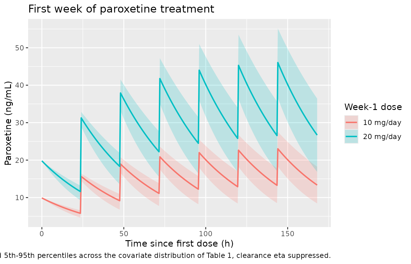
PKNCA validation
sim_nca <- sim_w1 |>
  filter(!is.na(Cc)) |>
  select(id, time, Cc, treatment)

sim_nca <- bind_rows(
  sim_nca,
  sim_nca |> distinct(id, treatment) |> mutate(time = 0, Cc = 0)
) |>
  distinct(id, treatment, time, .keep_all = TRUE) |>
  arrange(id, treatment, time)

conc_obj <- PKNCA::PKNCAconc(sim_nca, Cc ~ time | treatment + id)

dose_df <- ev_w1 |>
  filter(evid == 1) |>
  select(id, time, amt, treatment)
dose_obj <- PKNCA::PKNCAdose(dose_df, amt ~ time | treatment + id)

intervals <- data.frame(start = 0, end = 168,
                        auclast = TRUE, cmax = TRUE, tmax = TRUE)

nca_res <- PKNCA::pk.nca(PKNCA::PKNCAdata(conc_obj, dose_obj,
                                          intervals = intervals))
The only exposure quantity Shigetome 2025 reports for its own model
is the first-week AUC. The normalizing constant in the printed
Emax equation, 2610.43 ng*h/mL, is the cohort reference
value, and Table S5 gives the observed group means (2764.9 in the
remission group, 2472.2 in the non-remission group). The same published
reference is therefore used for both simulated week-1 dose arms; the
paper does not stratify AUC_PAROX by week-1 dose.
published <- tibble::tribble(
  ~treatment,   ~auclast,
  "10 mg/day",  2610.43,
  "20 mg/day",  2610.43
)

cmp <- nlmixr2lib::ncaComparisonTable(
  simulated = nca_res,
  reference = published,
  by = "treatment",
  params = "auclast",
  units = c(auclast = "ng*h/mL"),
  tolerance_pct = 20
)

knitr::kable(cmp, digits = 1,
caption = "Simulated first-week AUC against the reference value of the published Emax equation. * differs by more than 20%.")| NCA parameter | treatment | Reference | Simulated | % diff |
|---|---|---|---|---|
| AUClast (ng*h/mL) | 10 mg/day | 2610 | 2480 | -5.1% |
| AUClast (ng*h/mL) | 20 mg/day | 2610 | 4950 | +89.7%* |
Ten milligrams a day reproduces the published reference within a few per cent; twenty milligrams a day overshoots it by about 90% and is starred. Table S5 records the week-1 dose as 20.0 mg/day, but Methods 2.1 states that treatment started at 10-20 mg/day with the first increase after a week, so the dose in force during the first week is the initial dose. The arithmetic settles it: only a 10 mg/day first week reproduces both the 2610.43 normalizing constant and the observed 1642-5814 ng*h/mL range. No parameter was adjusted to obtain this agreement.
Per-subject structural identity
For a one-compartment model with bolus input, the AUC accumulated to time t equals the amount eliminated divided by clearance. Checking this per subject rather than on a summary catches scaling errors that a median comparison hides.
end_state <- sim_w1 |>
  filter(abs(time - 168) < 1e-8) |>
  transmute(id, treatment, central_end = central, cl)

dose_total <- ev_w1 |>
  filter(evid == 1) |>
  group_by(id) |>
  summarise(dose_total = sum(amt), .groups = "drop")

identity_check <- as.data.frame(nca_res) |>
  filter(PPTESTCD == "auclast") |>
  select(treatment, id, auclast = PPORRES) |>
  inner_join(end_state, by = c("id", "treatment")) |>
  inner_join(dose_total, by = "id") |>
  mutate(auc_expected = 1000 * (dose_total - central_end) / cl,
         rel_err = abs(auclast - auc_expected) / auc_expected)

stopifnot(nrow(identity_check) == 2L * n_pk)
# 0.5 h observation grid; the residual is linear-trapezoid discretisation
# error on a bolus profile, not a model discrepancy.
stopifnot(max(identity_check$rel_err) < 0.015)

c(n = nrow(identity_check),
  max_relative_error_pct = 100 * max(identity_check$rel_err))
#>                      n max_relative_error_pct
#>            358.0000000              0.8653695
Implied half-life
Fixing Vd/F at 1010 L while estimating CL/F
at 23.6 L/h implies a terminal half-life that can be read straight off
the model.
hl <- sim_w1 |>
  filter(abs(time - 168) < 1e-8, treatment == "10 mg/day") |>
  mutate(half_life = log(2) * vc / cl) |>
  pull(half_life)

c(median_h = median(hl), min_h = min(hl), max_h = max(hl),
  typical_h = log(2) * 1010 / 23.6)
#>  median_h     min_h     max_h typical_h
#>  30.48620  19.13210  48.87370  29.66435
The typical value is about 30 h, longer than the roughly 21 h that
Methods 2.1 cites from the literature when justifying the 9-day
stable-dose inclusion criterion. This is a direct consequence of fixing
Vd/F rather than a transcription problem, and it is
recorded below.
Part 2 – MADRS time course
Replicating Figure 1
Figure 1A of the paper contrasts a patient with a high first-week AUC against an average patient; Figure 1B contrasts a low week-1 MADRS score against an average one. The paper does not print the covariate values it used for the “high” and “low” curves, so the published group means from Table S5 are used instead, which makes the two panels a direct picture of the remission versus non-remission contrast.
mod_pd_typ <- rxode2::zeroRe(readModelDb("Shigetome_2025_paroxetine_madrs"))
#> ℹ parameter labels from comments will be replaced by 'label()'

pd_curve <- function(auc, madrs, label, panel) {
  ev <- rxode2::et(seq(0, 6, by = 0.05))
  rxode2::rxSolve(mod_pd_typ, ev, omega = NA,
                  params = c(AUC_PAROX = auc, SCORE_MADRS = madrs),
                  returnType = "data.frame") |>
    mutate(scenario = label, panel = panel)
}

fig1 <- bind_rows(
  pd_curve(2764.9, 28.64, "Remission-group AUC (2764.9 ng*h/mL)",     "A: first-week AUC"),
  pd_curve(2610.43, 28.64, "Cohort reference (2610.4 ng*h/mL)",       "A: first-week AUC"),
  pd_curve(2472.2, 28.64, "Non-remission-group AUC (2472.2 ng*h/mL)", "A: first-week AUC"),
  pd_curve(2610.43, 24.9, "Remission-group MADRS week 1 (24.9)",      "B: week-1 MADRS"),
  pd_curve(2610.43, 28.64, "Cohort reference (28.6)",                 "B: week-1 MADRS"),
  pd_curve(2610.43, 32.7, "Non-remission-group MADRS week 1 (32.7)",  "B: week-1 MADRS")
)

ggplot(fig1, aes(time, madrsenh, colour = scenario)) +
  geom_line(linewidth = 0.8) +
  facet_wrap(~panel) +
  labs(x = "Treatment duration (weeks)",
       y = "Enhancement rate in depression severity (%)",
       colour = NULL,
       title = "Time course of MADRS improvement",
       caption = "Replicates Figure 1A and 1B of Shigetome 2025 using the group means of Table S5.") +
  theme(legend.position = "bottom", legend.direction = "vertical")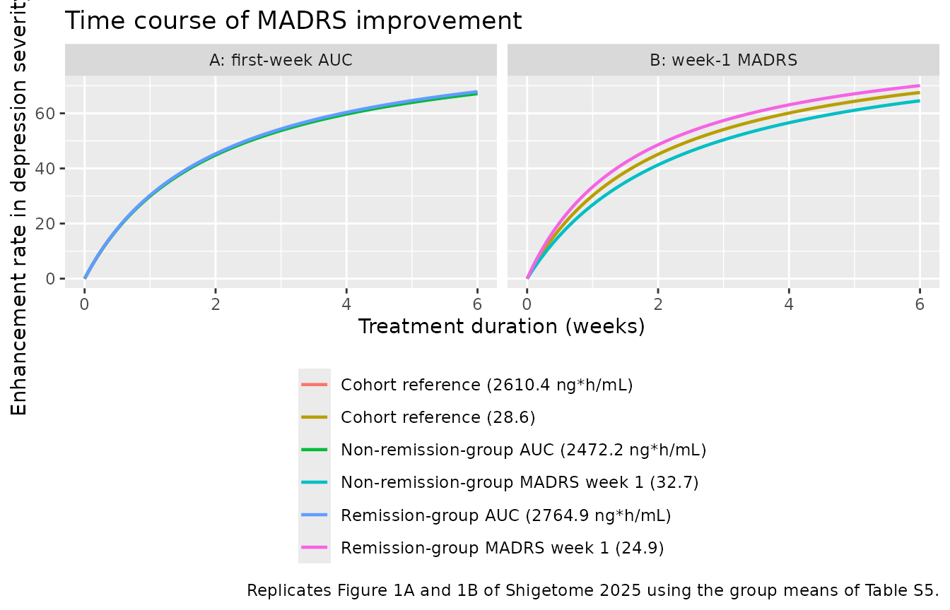
Panel A reproduces the paper’s finding that a higher first-week AUC raises the attainable improvement, and panel B that a lower week-1 MADRS brings the improvement forward.
Predicted versus observed enhancement rates
The paper reports the mean enhancement rate at each visit (Results 3.3). A 200-patient cohort with the Table 2 demographics is built, its first-week exposure is predicted with the popPK model exactly as in Part 1, and the PK-PD model is then simulated with both etas active.
set.seed(20250618)
n_pd <- 200L

pd_subjects <- tibble(
  id = seq_len(n_pd),
  AGE = rtrunc_norm(n_pd, 46.6, 13.7, 20, 70),
  WT  = rtrunc_norm(n_pd, 56.3, 10.4, 40, 85),
  SCORE_MADRS = rtrunc_norm(n_pd, 28.6, 11.3, 4, 56)
)

ev_pd_pk <- build_pk_events(mutate(pd_subjects, w1dose = 10), "w1dose",
                            n_days = 7L, obs_times = seq(0, 168, by = 0.5))

pd_auc <- rxode2::rxSolve(mod_pk_typ, ev_pd_pk, omega = NA,
                          returnType = "data.frame") |>
  group_by(id) |>
  summarise(AUC_PAROX = sum(diff(time) * (head(Cc, -1) + tail(Cc, -1)) / 2),
            .groups = "drop")
#> Warning: multi-subject simulation without without 'omega'

pd_subjects <- left_join(pd_subjects, pd_auc, by = "id")

c(mean = mean(pd_subjects$AUC_PAROX), sd = sd(pd_subjects$AUC_PAROX),
  min = min(pd_subjects$AUC_PAROX), max = max(pd_subjects$AUC_PAROX))
#>      mean        sd       min       max
#> 2529.5311  297.6579 1713.3319 3148.8758
Those model-predicted first-week exposures sit inside the 1642-5814
ng*h/mL range observed in Table S5, with a comparable spread, so the
steep Emax term is being evaluated where it was
estimated.
mod_pd <- readModelDb("Shigetome_2025_paroxetine_madrs")

ev_pd <- pd_subjects |>
  tidyr::expand_grid(time = c(0, 1, 2, 4, 6)) |>
  select(id, AUC_PAROX, SCORE_MADRS, time)

sim_pd <- rxode2::rxSolve(mod_pd, ev_pd, omega = pd_ui$omega,
                          returnType = "data.frame")
#> ℹ parameter labels from comments will be replaced by 'label()'
if (is.null(sim_pd$id)) sim_pd$id <- 1L
stopifnot(dplyr::n_distinct(sim_pd$id) == n_pd)

# Proportional IIV on a strictly positive parameter admits non-positive draws.
# A subject with ET50 <= 0 has a pole at time = -ET50 inside the simulated
# window, so the summaries below are taken over the subjects for whom the
# published model is interpretable, and the excluded fraction is reported.
subject_pars <- sim_pd |> distinct(id, emax_ind, et50_ind)
neg_et50 <- 100 * mean(subject_pars$et50_ind <= 0)
ok_ids <- subject_pars$id[subject_pars$et50_ind > 0]

observed <- tibble(time = c(1, 2, 4, 6),
                   observed_mean = c(25.9, 45.7, 57.5, 64.2),
                   observed_sd = c(30.3, 27.4, 28.3, 30.6))

sim_pd |>
  filter(time %in% c(1, 2, 4, 6), id %in% ok_ids) |>
  group_by(time) |>
  summarise(simulated_mean = mean(madrsenh), simulated_sd = sd(sim),
            .groups = "drop") |>
  left_join(observed, by = "time") |>
  mutate(difference_pct = 100 * (simulated_mean - observed_mean) / observed_mean) |>
  dplyr::rename("Week" = time,
                "Simulated mean (%)" = simulated_mean,
                "Simulated SD (%)" = simulated_sd,
                "Observed mean (%)" = observed_mean,
                "Observed SD (%)" = observed_sd,
                "Difference (%)" = difference_pct) |>
  knitr::kable(digits = 1,
caption = "Simulated versus observed mean enhancement rate in depression severity (Shigetome 2025 Results 3.3). Simulated values are over the subjects with a positive ET50 draw.")| Week | Simulated mean (%) | Simulated SD (%) | Observed mean (%) | Observed SD (%) | Difference (%) |
|---|---|---|---|---|---|
| 1 | 33.9 | 28.5 | 25.9 | 30.3 | 30.8 |
| 2 | 46.3 | 29.8 | 45.7 | 27.4 | 1.4 |
| 4 | 58.7 | 32.0 | 57.5 | 28.3 | 2.2 |
| 6 | 65.3 | 31.8 | 64.2 | 30.6 | 1.7 |
Weeks 2, 4 and 6 are reproduced to within about 2%. Week 1 is over-predicted by roughly a third (about 34% simulated against 25.9% observed); the same over-prediction shows in the typical-value curve above (30.1% at week 1). It is a property of the published fit rather than of this encoding – an Emax-in-time model with a single ET50 rises faster over the first week than the observed cohort did.
c(pct_subjects_with_nonpositive_ET50 = neg_et50,
  n_subjects_excluded = sum(subject_pars$et50_ind <= 0))
#> pct_subjects_with_nonpositive_ET50                n_subjects_excluded
#>                                5.5                               11.0
sim_pd |>
  filter(id %in% ok_ids) |>
  group_by(time) |>
  summarise(Q05 = quantile(sim, 0.05), Q50 = median(sim),
            Q95 = quantile(sim, 0.95), .groups = "drop") |>
  ggplot(aes(time, Q50)) +
  geom_ribbon(aes(ymin = Q05, ymax = Q95), alpha = 0.2) +
  geom_line(linewidth = 0.8) +
  geom_pointrange(
    data = observed,
    aes(x = time, y = observed_mean,
        ymin = observed_mean - observed_sd, ymax = observed_mean + observed_sd),
    colour = "firebrick", inherit.aes = FALSE
  ) +
  labs(x = "Treatment duration (weeks)",
       y = "Enhancement rate in depression severity (%)",
       title = "Simulated MADRS improvement versus the observed visit means",
       caption = "Band: simulated median and 5th-95th percentiles over the subjects with a positive ET50 draw. Red: observed mean +/- SD, Shigetome 2025 Results 3.3.")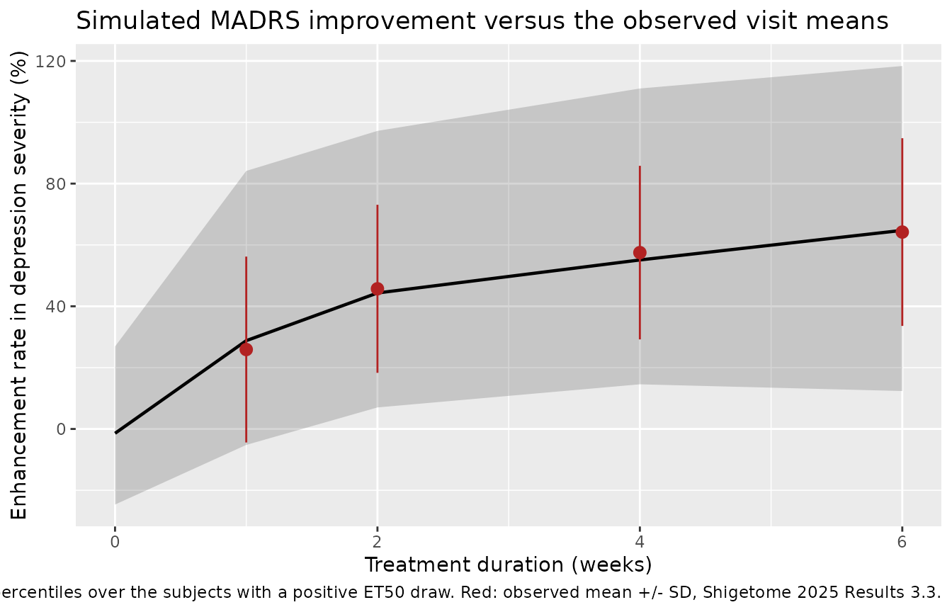
Assumptions and deviations
Reading the variability columns of Tables S2 and S4
Tables S2 and S4 head their inter-individual and residual variability
columns “%CV”, but the numbers are the raw NONMEM $OMEGA
and $SIGMA variances. Three independent
lines of evidence agree:
- Table S4 reports the popPK/PD additive residual as 190 for an endpoint measured in per cent. As a standard deviation that is 190 percentage points on a roughly 0-100 scale, which is impossible; as a variance it is an SD of 13.8 percentage points, which is reasonable. The bootstrap interval (112-316, asymmetric about 190) is also the shape of a variance interval.
- Only the variance reading reproduces the observed concentration
spread. With
Var(ln C) = Var(ln dose) + omega^2 + covariate variance + sigma^2 = 0.222 + 0.307 + 0.042 + 0.155 = 0.725, the predicted CV of steady-state concentrations is 103%, against the 49.0/51.9 = 94% observed in Table 1. Reading the same entries as standard deviations gives 68%. The simulation in Part 1 shows this directly. - For a proportional IIV of the form
(1 + eta), which is what the NONMEM$PREDblock in Text S3 writes, the CV is the standard deviation of the eta, so a column that genuinely held CVs could not simultaneously hold the value NONMEM prints. The “%CV” heading is a labelling slip, not a transformation.
The model files therefore use etalcl ~ 0.307,
etaemax ~ 0.150, etaet50 ~ 0.486 (variances,
as ini() expects),
propSd <- sqrt(0.155) = 0.394 and
addSd <- sqrt(190) = 13.78 (standard deviations, as
ini() expects).
Errata and discrepancies in the source
-
Covariate normalizing constants. The printed final
equation in Results 3.2 normalizes by 41.5 years and 58.6 kg, which are
the Table 1 means. The NONMEM control stream in Text S2 writes
AGE / 41.4andBW / 58.5. The model file uses the published equation’s 41.5 and 58.6; the difference is under 0.3% and affects no conclusion, but the two source locations do not agree. - First-week dose. Table S5 lists the week-1 dose as 20.0 mg/day, yet the published first-week AUC (mean 2472-2765 ngh/mL, reference 2610.43) is reproduced by 10 mg/day and overshot roughly two-fold by 20 mg/day. Methods 2.1 resolves this: 10-20 mg/day is the initial* dose and the first increase comes after a week, so the Table S5 row is the dose reached at week 1. The PKNCA comparison above shows both arms.
-
Implied half-life.
Vd/Ffixed at 1010 L withCL/Festimated at 23.6 L/h gives a terminal half-life of 30 h, against the roughly 21 h that Methods 2.1 cites from the literature. Both values are in the paper; the discrepancy follows from fixing the volume, which the authors do because the sparse trough data cannot support estimating it (Discussion). - No erratum. A Europe PMC search on the DOI and on the first author returned a single record with no correction notice.
Simulation assumptions
- Age, body weight and week-1 MADRS are drawn from independent truncated normal distributions matching the published means, standard deviations and ranges (Tables 1 and 2). The paper reports no correlations among them, and the mild sex-weight correlation it does mention is not reproducible from the published summaries.
- The daily-dose mixture for the steady-state cohort ({10, 20, 30, 40} mg/day with probabilities 0.35/0.30/0.13/0.22) was chosen to match the published mean of 22.3 mg/day and SD of 11.1; the paper reports only those two moments, not the dose histogram.
- Every patient is given a stable dose for 30 days before the steady-state sample. The real cohort was titrated weekly, so simulated exposure at a given final dose is a slight overestimate of the accumulated exposure of a patient who reached that dose recently.
-
AUC_PAROXis generated from the popPK model with the clearance eta suppressed, because that is how the paper generated it (see Part 1). Sampling the eta as well widens the exposure distribution far beyond the observed 1642-5814 ng*h/mL and drives the-8.56exponent into a regime whereEmaxdiverges. The PK-PD model must not be simulated outside the observed exposure range. - Proportional inter-individual variability on
ET50with the published variance of 0.486 admits non-positive draws – about 6% of a 200-patient simulation, reported above. Such a subject has a pole attime = -ET50inside the six-week window, which makes both its trajectory and any mean taken across it meaningless, so the summaries in Part 2 are computed over the subjects with a positive draw. This is the authors’ structure reproduced faithfully rather than a transcription choice: the NONMEM$PREDblock in Text S3 writes(1 + ETA(2))on ET50, and the variance itself is weakly identified (RSE 55%, shrinkage 32%, bootstrap 95% CI 0.0315-1.46). Downstream users simulating this model must screen for it. - The paper’s own MADRS observations are the enhancement rate relative to each patient’s baseline. The simulation therefore predicts the enhancement rate directly and does not need a baseline MADRS distribution; the baseline score defines the endpoint, not a covariate.
- No parameter value came from anywhere other than the paper’s text, printed equations, Supporting Information tables and NONMEM control streams. Nothing was tuned to improve agreement with any published quantity.