Belantamab mafodotin ADC, total antibody and cys-mcMMAF (Rathi 2021)
Source:vignettes/articles/Rathi_2021_belantamab.Rmd
Rathi_2021_belantamab.RmdModel and source
- Citation: Rathi C, Collins J, Struemper H, Opalinska J, Jewell RC, Ferron-Brady G. Population pharmacokinetics of belantamab mafodotin, a BCMA-targeting agent in patients with relapsed/refractory multiple myeloma. CPT Pharmacometrics Syst Pharmacol. 2021;10(8):851-863. doi:10.1002/psp4.12660
- Description: Sequential three-analyte population PK model for the antibody-drug conjugate belantamab mafodotin in patients with relapsed/refractory multiple myeloma (Rathi 2021; DREAMM-1 and DREAMM-2). The ADC (output Cc, ug/mL) follows a linear two-compartment model with a sigmoidal time-varying clearance and covariate effects of baseline body weight, albumin, soluble BCMA, IgG, sex, dose below 1 mg/kg and study. First-order deconjugation (kdec) converts ADC into naked antibody, which shares the ADC distribution parameters; total antibody (output Cc_tab, nM) is the sum of ADC and naked antibody times an assay correction factor. The cys-mcMMAF payload (output Cc_mcmmaf, nM) follows a linear two-compartment model fed by the ADC clearance flux times an empirical drug-to-antibody ratio that decays exponentially with time after each dose and resets at every dose, with inter-occasion variability on its clearance and central volume.
- Article (open access): https://doi.org/10.1002/psp4.12660
- Supplement (Tables S1-S4 and the NONMEM control streams of all three models in the Supplementary Methods): available from the article page.
Rathi 2021 fitted three models sequentially. The ADC model was fitted first. The total-antibody and cys-mcMMAF models were then fitted with the ADC individual post hoc parameters as fixed inputs. Neither later model can be used without the ADC model, so the three are packaged as one model with three outputs:
| Output | Analyte | Units | Sub-model |
|---|---|---|---|
Cc |
belantamab mafodotin ADC | ug/mL | Table 1 |
Cc_tab |
total antibody (ADC + naked antibody) | nM | Table S3 |
Cc_mcmmaf |
cys-mcMMAF payload | nM | Table S4 |
The dose (mg of ADC) goes into central. In the control
streams 1 nM of ADC is 152.1 ng/mL and 1 nM of cys-mcMMAF is 1.045
ng/mL; the model applies the same factors.
Population
Rathi 2021 pooled 291 patients with relapsed/refractory multiple myeloma from DREAMM-1 (phase I, n = 73, 0.03-4.6 mg/kg as a 1-h infusion every 3 weeks) and DREAMM-2 (phase II, n = 218, 2.5 or 3.4 mg/kg as a 30-min infusion every 3 weeks; 24 of the 3.4 mg/kg patients received the lyophilised presentation). The median age was 65 (34-89) years and the median body weight 74.0 (42.4-130) kg. 54% were men and 83% White. Median baseline albumin was 39.0 g/L, sBCMA 80.0 ng/mL and IgG 8.50 g/L (Table S2). The typical patient used for the paper’s exposure calculations is a 65-year-old man from DREAMM-2 weighing 75 kg, with sBCMA 100 ng/mL, IgG 10 g/L and albumin 40 g/L, receiving 2.5 mg/kg.
The same information is available programmatically via
readModelDb("Rathi_2021_belantamab")()$population.
Source trace
Table 1 prints the ADC estimates to two decimals. The unrounded final
estimates appear as the fixed $THETA values in the
total-mAb and cys-mcMMAF control streams (Supplementary Methods), and
those are the values used. Each rounds to its Table 1 value.
| Equation / parameter | Value | Source location |
|---|---|---|
| ADC two-compartment ODE, dose into central | n/a | Supplementary Methods ADC control stream
(ADVAN3 TRANS4) |
lcl (CL0) |
log(0.936) L/day | Table 1 TVCL 0.94; control stream THETA(1) |
lvc (V1, female) |
log(4.47) L | Table 1 TVV1; THETA(2) |
lq |
log(0.781) L/day | Table 1 TVQ 0.78; THETA(3) |
lvp |
log(5.96) L | Table 1 TVV2; THETA(4) |
time-varying CL
exp(IMAX t^GAMMA / (TI50^GAMMA + t^GAMMA))
|
n/a | Results equation; control stream CLT
|
cl_time_max (IMAX, additive eta) |
-0.327 | Table 1 -0.33; THETA(5) |
lcl_t50 (TI50) |
log(53.9) day | Table 1; THETA(6) |
lcl_time_hill (GAMMA) |
log(4.30) | Table 1; THETA(7) |
e_wt_cl, e_wt_vc
|
0.507, 0.500 | Table 1; THETA(17), THETA(10) |
e_alb_cl, e_alb_vc
|
-0.972, -0.471 | Table 1; THETA(12), THETA(13) |
e_sexm_vc |
1.14 | Table 1; THETA(14), applied as THETA**SEX with SEX = 1
for males |
e_sbcma_cl, e_igg_cl
|
0.126, 0.127 | Table 1; THETA(15), THETA(16) |
e_dose_low_vp, e_dose_low_cl
|
0.129, 0.623 | Table 1; THETA(20), THETA(21) |
e_study_dreamm1_vc,
e_study_dreamm1_cl
|
0.66, 0.608 | Table 1; THETA(22), THETA(23) |
| ADC IIV (CL, V1, Q, V2, IMAX, TI50) | 35.0, 14.6, 37.8, 46.8, 123, 30.1 percent CV | Table 1 |
expSd |
sqrt(0.019) | Table 1 ‘additive SIGMA on log scale’ |
| naked antibody ODE: ADC loses CL/V1, kdec of it to naked antibody, which is eliminated at CL/V1 - kdec | n/a | Supplementary Methods total-mAb $DES
|
lkdec, e_dose_low_kdec
|
log(0.0590) /day, 0.0001 (held constant) | Table S3 |
| total antibody = (ADC + naked) x CORR | n/a | Table S3 residual-error equation; Results |
lcal_slope_tab (CORR) |
log(1.14) | Table S3 |
e_study_dreamm1_cal_slope_tab,
e_dose_low_cal_slope_tab
|
0.848, 0.846 | Table S3 |
| total-antibody IIV (Kdec, CORR) | 38.8, 7.58 percent CV | Table S3 |
expSd_tab |
sqrt(0.0516) | Table S3 |
cys-mcMMAF input (CL/V1) x A_ADC x DAR(t)
|
n/a | Supplementary Methods cys-mcMMAF $DES
|
DAR(t) = DAR0 exp(-RATE x TAD), reset at each dose |
n/a | Results equation; control stream DARF
|
lkdar (RATE-DAR) |
log(0.067) /day | Table S4 |
mdar (DAR0) |
3.93 (held constant) | back-solved from the Results cys-mcMMAF Cavg (see Assumptions) |
lcl_mcmmaf, lvc_mcmmaf
|
log(648) L/day, log(30.4) L | Table S4 |
lk12_mcmmaf (K34), lk21_mcmmaf (K43) |
log(74.9), log(5.62) /day | Table S4 |
e_sbcma_vc_mcmmaf, e_igg_vc_mcmmaf
|
0.131, 0.154 | Table S4 |
e_study_dreamm1_vc_mcmmaf |
0.507, as (1 + theta) | Table S4; control stream VSTUDY
|
| cys-mcMMAF IIV block (CL, V3, K43) | 0.100; 0.112, 0.260; 0, 0.257, 0.956 | Table S4 |
| cys-mcMMAF IOV (CL, V3), OCC 1, 2, 3, > 3 | 0.100, 0.185 | Table S4; control stream IOV, IOV2
|
DREAMM-1 VALA recalibration
1.486 x C - 8.360 pg/mL
|
cal_slope_vala 1.486, cal_int_vala -0.008
nM |
Methods equation; control stream SLP,
INT
|
| cys-mcMMAF residual error, DREAMM-2 | prop sqrt(0.051), add sqrt(0.0002) nM | Table S4 |
| cys-mcMMAF residual error, DREAMM-1 | prop sqrt(0.0851), add sqrt(0.0009) nM | Table S4 |
mod <- readModelDb("Rathi_2021_belantamab")
ui <- rxode2::rxode(mod)
#> ℹ parameter labels from comments will be replaced by 'label()'
#> Warning: some etas defaulted to non-mu referenced, possible parsing error: etaiov_vc_mcmmaf_4, etaiov_vc_mcmmaf_3, etaiov_vc_mcmmaf_2, etaiov_vc_mcmmaf_1, etaiov_cl_mcmmaf_4, etaiov_cl_mcmmaf_3, etaiov_cl_mcmmaf_2, etaiov_cl_mcmmaf_1
#> as a work-around try putting the mu-referenced expression on a simple line
Typical-patient exposures
Rathi 2021 (Results, ‘Typical patient and impact of covariates on exposure measures’) reports the cycle-1 exposures of the typical DREAMM-2 patient after 2.5 mg/kg: ADC Cmax 36.5, Cavg 7.76 and Ctau 2.22 ug/mL, and cys-mcMMAF Cmax 917 and Cavg 217 pg/mL. The values are stated to be 1.36-fold higher at 3.4 mg/kg. Below, the typical patient is simulated without random effects and the exposures are computed with PKNCA over the 21-day cycle.
typ_cov <- data.frame(
  WT = 75, ALB = 40, SBCMA = 100, IGG = 10, SEXF = 0,
  STUDY_DREAMM1 = 0, DOSE_LOW = 0, OCC = 1
)
obs_grid <- sort(unique(c(seq(0, 1, by = 0.005), seq(1, 21, by = 0.05))))

make_typical <- function(id, dose_mgkg, cov = typ_cov, inf_h = 0.5) {
  amt <- dose_mgkg * cov$WT
  dose <- data.frame(
    id = id, time = 0, amt = amt, rate = amt / (inf_h / 24),
    evid = 1L, cmt = "central", dvid = NA_integer_
  )
  obs <- data.frame(
    id = id, time = obs_grid, amt = NA_real_, rate = NA_real_,
    evid = 0L, cmt = "central", dvid = 1L
  )
  dplyr::bind_rows(dose, obs) |>
    dplyr::mutate(treatment = paste(dose_mgkg, "mg/kg")) |>
    cbind(cov[rep(1, nrow(dose) + nrow(obs)), , drop = FALSE])
}

typ_events <- dplyr::bind_rows(
  make_typical(1L, 2.5),
  make_typical(2L, 3.4)
)
typ <- rxode2::rxSolve(
  mod, typ_events,
  omega = NA, sigma = NA, useLinCmt = FALSE,
  keep = "treatment", returnType = "data.frame"
)
#> ℹ parameter labels from comments will be replaced by 'label()'
#> Warning: some etas defaulted to non-mu referenced, possible parsing error: etaiov_vc_mcmmaf_4, etaiov_vc_mcmmaf_3, etaiov_vc_mcmmaf_2, etaiov_vc_mcmmaf_1, etaiov_cl_mcmmaf_4, etaiov_cl_mcmmaf_3, etaiov_cl_mcmmaf_2, etaiov_cl_mcmmaf_1
#> as a work-around try putting the mu-referenced expression on a simple line
nca_one <- function(sim, conc_col) {
  conc <- sim |>
    dplyr::filter(!is.na(.data[[conc_col]])) |>
    dplyr::transmute(id, time, treatment, Cc = .data[[conc_col]]) |>
    dplyr::distinct(id, treatment, time, .keep_all = TRUE)
  dose <- typ_events |>
    dplyr::filter(evid == 1) |>
    dplyr::select(id, time, amt, treatment)
  res <- PKNCA::pk.nca(PKNCA::PKNCAdata(
    PKNCA::PKNCAconc(conc, Cc ~ time | treatment + id),
    PKNCA::PKNCAdose(dose, amt ~ time | treatment + id),
    intervals = data.frame(start = 0, end = 21, cmax = TRUE, cav = TRUE, clast.obs = TRUE)
  ))
  res
}

nca_adc <- nca_one(typ, "Cc")
# cys-mcMMAF reported in pg/mL: nM x 1045
typ$Cc_mcmmaf_pgml <- typ$Cc_mcmmaf * 1045
nca_mmaf <- nca_one(typ, "Cc_mcmmaf_pgml")

pub_adc <- tibble::tribble(
  ~treatment, ~cmax, ~cav, ~clast.obs,
  "2.5 mg/kg", 36.5, 7.76, 2.22,
  "3.4 mg/kg", 36.5 * 1.36, 7.76 * 1.36, 2.22 * 1.36
)
pub_mmaf <- tibble::tribble(
  ~treatment, ~cmax, ~cav,
  "2.5 mg/kg", 917, 217,
  "3.4 mg/kg", 917 * 1.36, 217 * 1.36
)

cmp_adc <- nlmixr2lib::ncaComparisonTable(
  simulated = nca_adc, reference = pub_adc, by = "treatment",
  units = c(cmax = "ug/mL", cav = "ug/mL", clast.obs = "ug/mL"),
  tolerance_pct = 20
)
knitr::kable(cmp_adc, caption = "ADC cycle-1 exposures of the typical DREAMM-2 patient: simulated vs. Rathi 2021 Results (3.4 mg/kg reference = 1.36 x the 2.5 mg/kg value, as stated in the paper). Ctau is the concentration at day 21. * differs from reference by >20%.")| NCA parameter | treatment | Reference | Simulated | % diff |
|---|---|---|---|---|
| Cmax (ug/mL) | 2.5 mg/kg | 36.5 | 36.6 | +0.3% |
| Cmax (ug/mL) | 3.4 mg/kg | 49.6 | 49.8 | +0.3% |
| Clast (ug/mL) | 2.5 mg/kg | 2.22 | 2.22 | -0.1% |
| Clast (ug/mL) | 3.4 mg/kg | 3.02 | 3.01 | -0.1% |
| Cavg (ug/mL) | 2.5 mg/kg | 7.76 | 7.75 | -0.1% |
| Cavg (ug/mL) | 3.4 mg/kg | 10.6 | 10.5 | -0.1% |
cmp_mmaf <- nlmixr2lib::ncaComparisonTable(
  simulated = nca_mmaf, reference = pub_mmaf, by = "treatment",
  params = c("cmax", "cav"),
  units = c(cmax = "pg/mL", cav = "pg/mL"),
  tolerance_pct = 20
)
knitr::kable(cmp_mmaf, caption = "cys-mcMMAF cycle-1 exposures of the typical DREAMM-2 patient: simulated vs. Rathi 2021 Results. * differs from reference by >20%.")| NCA parameter | treatment | Reference | Simulated | % diff |
|---|---|---|---|---|
| Cmax (pg/mL) | 2.5 mg/kg | 917 | 838 | -8.7% |
| Cmax (pg/mL) | 3.4 mg/kg | 1250 | 1140 | -8.7% |
| Cavg (pg/mL) | 2.5 mg/kg | 217 | 217 | -0.0% |
| Cavg (pg/mL) | 3.4 mg/kg | 295 | 295 | -0.0% |
nca_val <- function(res, code, trt) {
  d <- as.data.frame(res)
  d$PPORRES[d$PPTESTCD == code & d$treatment == trt]
}
pct <- function(sim, ref) 100 * (sim - ref) / ref
# The typical patient is deterministic, so these gates are tight. The ADC model
# is transcribed directly; a mis-typed CL, V1 or covariate centre moves these
# by far more than 2%.
stopifnot(
  abs(pct(nca_val(nca_adc, "cmax", "2.5 mg/kg"), 36.5)) < 2,
  abs(pct(nca_val(nca_adc, "cav", "2.5 mg/kg"), 7.76)) < 2,
  abs(pct(nca_val(nca_adc, "clast.obs", "2.5 mg/kg"), 2.22)) < 2,
  # cys-mcMMAF Cavg is the quantity DAR0 was back-solved from.
  abs(pct(nca_val(nca_mmaf, "cav", "2.5 mg/kg"), 217)) < 2,
  # cys-mcMMAF Cmax is ~9% below the printed 917 pg/mL; see Assumptions.
  abs(pct(nca_val(nca_mmaf, "cmax", "2.5 mg/kg"), 917)) < 15,
  # Linear in dose above 1 mg/kg.
  abs(nca_val(nca_adc, "cmax", "3.4 mg/kg") / nca_val(nca_adc, "cmax", "2.5 mg/kg") - 1.36) < 0.001
)
Half-life and time-varying clearance (Figure 3)
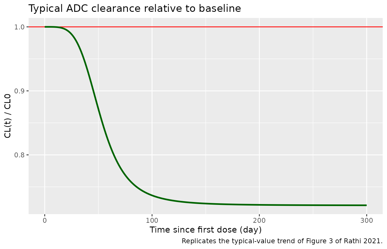
The Results state an initial typical ADC CL of 0.94 L/day with a half-life of 11.5 days, falling by 28% over time to give a half-life of 14.3 days. The terminal half-life follows from the two-compartment micro-constants at t = 0 and at t much greater than TI50. The printed half-lives are reproduced with the typical values themselves, i.e. with V1 = 4.47 L, which is the female reference (the male factor of 1.14 is not applied). For the typical man the half-lives are about 0.3-0.5 days longer.
p <- ui$theta
q <- exp(p[["lq"]])
vp <- exp(p[["lvp"]])
beta_hl <- function(cl, vc) {
  k10 <- cl / vc
  k12 <- q / vc
  k21 <- q / vp
  s <- k10 + k12 + k21
  beta <- (s - sqrt(s^2 - 4 * k10 * k21)) / 2
  log(2) / beta
}
cl0 <- exp(p[["lcl"]])
cl_inf <- cl0 * exp(p[["cl_time_max"]])
vc_ref <- exp(p[["lvc"]])
vc_male <- vc_ref * p[["e_sexm_vc"]]
hl <- rbind(
  `typical values (V1 = 4.47 L)` = c(initial = beta_hl(cl0, vc_ref), late = beta_hl(cl_inf, vc_ref)),
  `typical man (V1 x 1.14)` = c(initial = beta_hl(cl0, vc_male), late = beta_hl(cl_inf, vc_male))
)
knitr::kable(hl, digits = 2, caption = "ADC terminal half-life (day) at the start of treatment and after the full time-varying CL change. Rathi 2021: 11.5 and 14.3 days.")| initial | late | |
|---|---|---|
| typical values (V1 = 4.47 L) | 11.49 | 14.30 |
| typical man (V1 x 1.14) | 11.78 | 14.77 |
round(100 * (1 - exp(p[["cl_time_max"]])), 1)
#> [1] 27.9
stopifnot(
  abs(hl[1, "initial"] - 11.5) < 0.1,
  abs(hl[1, "late"] - 14.3) < 0.1,
  abs(100 * (1 - exp(p[["cl_time_max"]])) - 28) < 1
)
# Replicates the typical-value curve of Figure 3 of Rathi 2021 (ADC CL
# relative to baseline vs. time). Figure 3 itself shows individual post hoc
# estimates with a LOESS line.
tibble(time = seq(0, 300, by = 1)) |>
  mutate(ratio = exp(p[["cl_time_max"]] * time^exp(p[["lcl_time_hill"]]) /
    (exp(p[["lcl_t50"]])^exp(p[["lcl_time_hill"]]) + time^exp(p[["lcl_time_hill"]])))) |>
  ggplot(aes(time, ratio)) +
  geom_hline(yintercept = 1, colour = "red") +
  geom_line(colour = "darkgreen", linewidth = 1) +
  labs(
    x = "Time since first dose (day)", y = "CL(t) / CL0",
    title = "Typical ADC clearance relative to baseline",
    caption = "Replicates the typical-value trend of Figure 3 of Rathi 2021."
  )
Covariate effects on exposure (Figure 5)
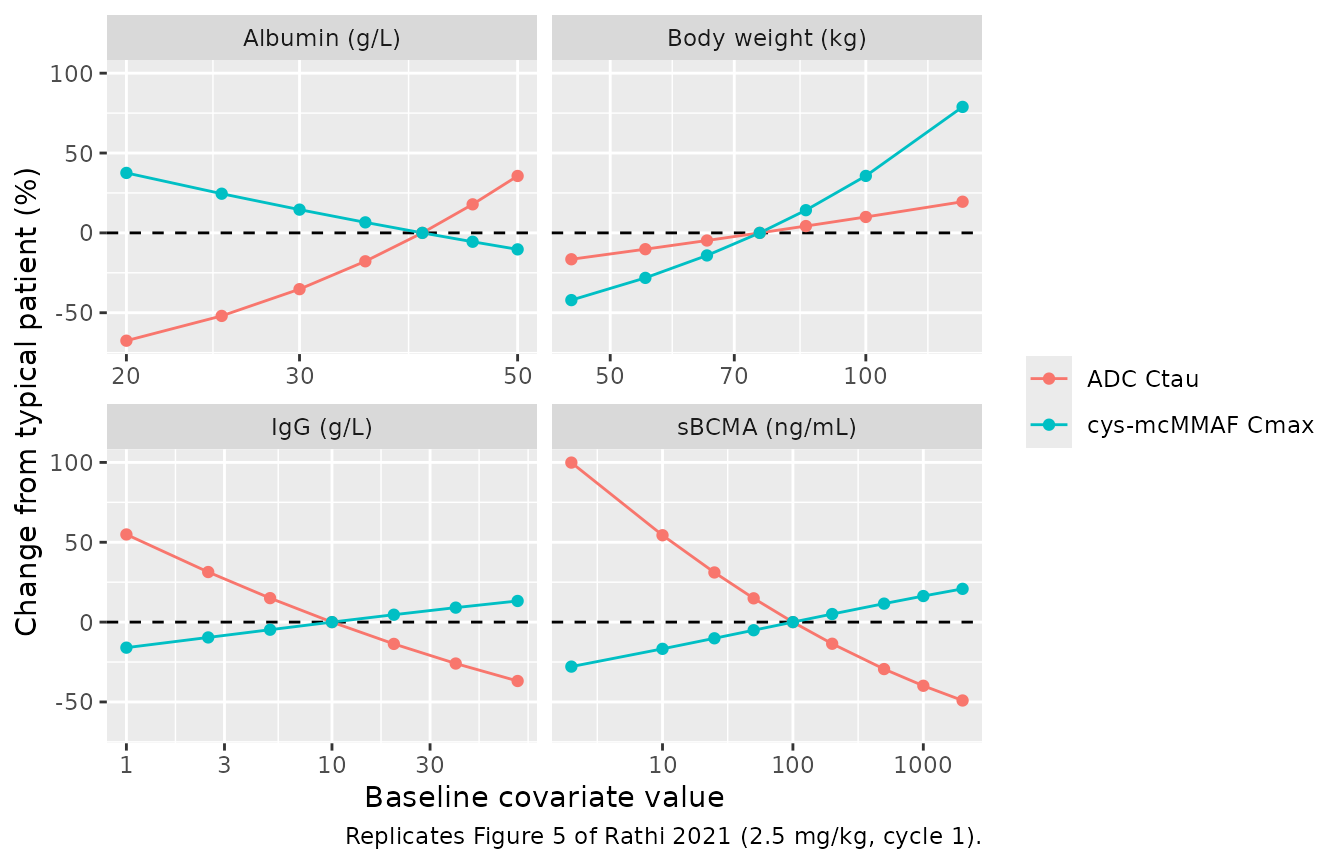
The Results state that a patient with a high baseline sBCMA of 500 ng/mL would have a 35% lower ADC Ctau than the typical patient. The figure below sweeps each continuous covariate of the typical patient across its observed range, holding the others at their typical values, as in Figure 5.
sweep <- dplyr::bind_rows(
  tibble(covariate = "sBCMA (ng/mL)", value = c(2, 10, 25, 50, 100, 200, 500, 1000, 2000)),
  tibble(covariate = "IgG (g/L)", value = c(1, 2.5, 5, 10, 20, 40, 80)),
  tibble(covariate = "Albumin (g/L)", value = c(20, 25, 30, 35, 40, 45, 50)),
  tibble(covariate = "Body weight (kg)", value = c(45, 55, 65, 75, 85, 100, 130))
) |>
  mutate(id = dplyr::row_number())

sweep_events <- lapply(seq_len(nrow(sweep)), function(i) {
  cov <- typ_cov
  col <- c(
    "sBCMA (ng/mL)" = "SBCMA", "IgG (g/L)" = "IGG",
    "Albumin (g/L)" = "ALB", "Body weight (kg)" = "WT"
  )[[sweep$covariate[i]]]
  cov[[col]] <- sweep$value[i]
  make_typical(sweep$id[i], 2.5, cov = cov)
}) |>
  dplyr::bind_rows()
stopifnot(!anyDuplicated(unique(sweep_events[, c("id", "time", "evid")])))

sweep_sim <- rxode2::rxSolve(
  mod, sweep_events,
  omega = NA, sigma = NA, useLinCmt = FALSE, returnType = "data.frame"
)
ref_ctau <- typ |> filter(treatment == "2.5 mg/kg", time == 21) |> pull(Cc)
ref_mmaf <- max(typ$Cc_mcmmaf[typ$treatment == "2.5 mg/kg"])
sweep_res <- sweep_sim |>
  group_by(id) |>
  summarise(ctau = Cc[time == 21], cmax_mmaf = max(Cc_mcmmaf), .groups = "drop") |>
  left_join(sweep, by = "id") |>
  mutate(
    `ADC Ctau` = 100 * (ctau / ref_ctau - 1),
    `cys-mcMMAF Cmax` = 100 * (cmax_mmaf / ref_mmaf - 1)
  )

sweep_res |>
  pivot_longer(c(`ADC Ctau`, `cys-mcMMAF Cmax`), names_to = "measure", values_to = "pct") |>
  ggplot(aes(value, pct, colour = measure)) +
  geom_hline(yintercept = 0, linetype = 2) +
  geom_line() +
  geom_point() +
  facet_wrap(~covariate, scales = "free_x") +
  scale_x_log10() +
  labs(
    x = "Baseline covariate value", y = "Change from typical patient (%)",
    colour = NULL,
    caption = "Replicates Figure 5 of Rathi 2021 (2.5 mg/kg, cycle 1)."
  )
pct_sbcma <- sweep_res |>
  filter(covariate == "sBCMA (ng/mL)") |>
  select(value, `ADC Ctau`)
pct_sbcma |>
  dplyr::rename("Baseline sBCMA (ng/mL)" = value, "ADC Ctau change (%)" = `ADC Ctau`) |>
knitr::kable(digits = 1, caption = "Percent change in ADC Ctau from the typical patient (sBCMA 100 ng/mL).")| Baseline sBCMA (ng/mL) | ADC Ctau change (%) |
|---|---|
| 2 | 99.9 |
| 10 | 54.4 |
| 25 | 31.1 |
| 50 | 14.9 |
| 100 | 0.0 |
| 200 | -13.5 |
| 500 | -29.4 |
| 1000 | -39.9 |
| 2000 | -49.1 |
pct_500 <- pct_sbcma$`ADC Ctau`[pct_sbcma$value == 500]
# The model gives about -29% at 500 ng/mL against the -35% stated in the
# Results (see Assumptions). The gate pins the deterministic model value, which
# depends only on the CL exponent 0.126 and the two-compartment disposition.
stopifnot(abs(pct_500 - (-29.4)) < 1)
The model gives a -29% change in ADC Ctau at an sBCMA of 500 ng/mL, against the 35% decrease stated in the Results. It gives about +50% at an sBCMA near 10 ng/mL, which matches the stated +50% for a very low baseline sBCMA. The sBCMA exponent on CL is printed identically in Table 1 and the control stream (0.126), so the maintainers record the 500 ng/mL difference as a deviation between the model and the paper’s text, not a transcription error.
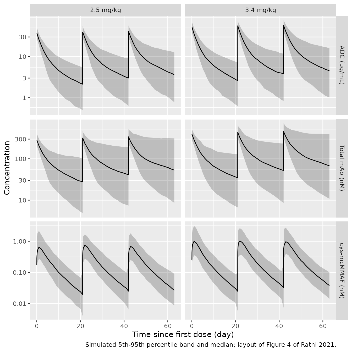
Virtual DREAMM-2 cohort
Observed data are not public. The virtual cohort draws baseline
covariates from distributions centred on the Table S2 medians and
bounded by the reported ranges: body weight log-normal (median 74 kg),
albumin normal (median 39 g/L), sBCMA and IgG log-normal (medians 80
ng/mL and 8.5 g/L, wide spread to cover the 1.95-2030 ng/mL and 0.3-99.7
g/L ranges), and 46% female. Two arms of 200 patients receive 2.5 or 3.4
mg/kg as a 30-min infusion every 3 weeks for three cycles.
OCC is the cycle number on every record, so each cycle
draws its own cys-mcMMAF inter-occasion deviation.
set.seed(2021)
rxode2::rxSetSeed(2021)
n_arm <- 200
make_cohort <- function(n, dose_mgkg, id_offset) {
  subj <- tibble(
    id = id_offset + seq_len(n),
    WT = pmin(pmax(exp(rnorm(n, log(74), 0.2)), 42.4), 130),
    ALB = pmin(pmax(rnorm(n, 39, 5), 19), 50),
    SBCMA = pmin(pmax(exp(rnorm(n, log(80), 1.2)), 1.95), 2030),
    IGG = pmin(pmax(exp(rnorm(n, log(8.5), 1.0)), 0.3), 99.7),
    SEXF = rbinom(n, 1, 0.46),
    STUDY_DREAMM1 = 0L,
    DOSE_LOW = 0L,
    treatment = paste(dose_mgkg, "mg/kg")
  )
  doses <- subj |>
    tidyr::crossing(time = c(0, 21, 42)) |>
    mutate(
      amt = dose_mgkg * WT, rate = amt / (0.5 / 24),
      evid = 1L, cmt = "central", dvid = NA_integer_
    )
  obs_t <- sort(unique(c(
    outer(c(0, 21, 42), c(0.5, 1, 2, 4, 8, 24, 72, 168, 336) / 24, "+"),
    seq(0, 63, by = 1)
  )))
  obs <- subj |>
    tidyr::crossing(time = obs_t) |>
    mutate(amt = NA_real_, rate = NA_real_, evid = 0L, cmt = "central", dvid = 1L)
  dplyr::bind_rows(doses, obs) |>
    mutate(OCC = pmin(floor(time / 21) + 1, 3)) |>
    arrange(id, time, desc(evid))
}
events <- dplyr::bind_rows(
  make_cohort(n_arm, 2.5, 0L),
  make_cohort(n_arm, 3.4, n_arm)
)
stopifnot(!anyDuplicated(unique(events[, c("id", "time", "evid")])))

sim <- rxode2::rxSolve(
  mod, events,
  useLinCmt = FALSE, keep = "treatment", returnType = "data.frame"
)
# Replicates the layout of Figure 4 of Rathi 2021 (VPC by analyte and dose):
# 5th, 50th and 95th percentiles of the simulated individual predictions
# (no residual error) over the first three cycles.
vpc <- sim |>
  select(id, time, treatment, ADC = Cc, `Total mAb` = Cc_tab, `cys-mcMMAF` = Cc_mcmmaf) |>
  pivot_longer(c(ADC, `Total mAb`, `cys-mcMMAF`), names_to = "analyte", values_to = "conc") |>
  filter(conc > 0) |>
  group_by(analyte, treatment, time) |>
  summarise(
    q05 = quantile(conc, 0.05), q50 = median(conc), q95 = quantile(conc, 0.95),
    .groups = "drop"
  ) |>
  mutate(analyte = factor(analyte, c("ADC", "Total mAb", "cys-mcMMAF"),
    c("ADC (ug/mL)", "Total mAb (nM)", "cys-mcMMAF (nM)")))

ggplot(vpc, aes(time, q50)) +
  geom_ribbon(aes(ymin = q05, ymax = q95), alpha = 0.25) +
  geom_line() +
  facet_grid(analyte ~ treatment, scales = "free_y") +
  scale_y_log10() +
  labs(
    x = "Time since first dose (day)", y = "Concentration",
    caption = "Simulated 5th-95th percentile band and median; layout of Figure 4 of Rathi 2021."
  )
c1 <- sim |>
  filter(time <= 21) |>
  group_by(id, treatment) |>
  summarise(
    cmax_adc = max(Cc), ctau_adc = Cc[time == 21][1],
    cmax_mmaf_pgml = max(Cc_mcmmaf) * 1045, .groups = "drop"
  )
c1_summary <- c1 |>
  group_by(treatment) |>
  summarise(across(c(cmax_adc, ctau_adc, cmax_mmaf_pgml), median), .groups = "drop")
knitr::kable(
  c1_summary |>
    dplyr::rename(
      "Dose" = treatment, "Median ADC Cmax (ug/mL)" = cmax_adc,
      "Median ADC Ctau (ug/mL)" = ctau_adc, "Median cys-mcMMAF Cmax (pg/mL)" = cmax_mmaf_pgml
    ),
  digits = 2, caption = "Cycle-1 medians of the virtual DREAMM-2 cohort."
)| Dose | Median ADC Cmax (ug/mL) | Median ADC Ctau (ug/mL) | Median cys-mcMMAF Cmax (pg/mL) |
|---|---|---|---|
| 2.5 mg/kg | 37.58 | 2.13 | 687.91 |
| 3.4 mg/kg | 52.82 | 2.59 | 1066.26 |
# Centre-of-distribution gates against the typical patient. The covariate
# draws are centred near the typical patient, so the cohort median sits
# within tens of percent of the typical value; a mis-transcribed CL, volume,
# dose or unit moves it by far more. Over four seeds the 2.5 mg/kg medians
# were 37.7-38.7 ug/mL (ADC Cmax), 1.92-2.22 ug/mL (ADC Ctau) and 699-831
# pg/mL (cys-mcMMAF Cmax, below the typical value because of the large V3 and
# K43 variability), all well inside these bounds.
med <- function(col, trt) c1_summary[[col]][c1_summary$treatment == trt]
stopifnot(
  abs(pct(med("cmax_adc", "2.5 mg/kg"), 36.5)) < 20,
  abs(pct(med("ctau_adc", "2.5 mg/kg"), 2.22)) < 35,
  abs(pct(med("cmax_mmaf_pgml", "2.5 mg/kg"), 917)) < 35
)
Assumptions and deviations
-
Product DAR0 back-solved. The cys-mcMMAF input is
the ADC clearance flux times an empirical DAR that resets to the
drug-product value DAR0 at every dose. The control stream reads DAR0
from a dataset column, and no numeric value appears in the paper, its
supplement or the control streams. The model output is linear in DAR0,
so the maintainers back-solved it from the typical-patient cys-mcMMAF
Cavg of 217 pg/mL (Results). That gives
mdar = 3.93, carried as a fixed parameter. Cavg was chosen over Cmax because it is an AUC-based measure and less sensitive to the sampling grid. Back-solving from the printed Cmax of 917 pg/mL would give 4.30 instead. The ratio of the two printed values, 917/217 = 4.23, cannot be reached with the printed Table S4 parameters, whose Cmax/Cavg ratio is 3.86 at any DAR0, so no single DAR0 matches both. Holding the DAR constant between the paper’s nominal sampling times, as NONMEM does for$PKquantities, gives a ratio of 3.71 and does not resolve the difference either. Withmdar = 3.93, the simulated typical cys-mcMMAF Cmax is about 9% below the printed value. Users with a known lot DAR can overridemdarviaini(). - sBCMA effect at 500 ng/mL. The Results state that a baseline sBCMA of 500 ng/mL lowers ADC Ctau by 35%. The model, using the printed CL exponent 0.126, gives about 29%. The difference is kept, not tuned.
- Half-life reference. The printed half-lives of 11.5 and 14.3 days match the typical values with V1 = 4.47 L, i.e. without the male V1 factor, while the printed typical-patient exposures include it.
- Unrounded ADC estimates. Table 1 prints two decimals. The model uses the values the authors held constant in the downstream control streams (e.g. CL 0.936, IMAX -0.327), which round to Table 1.
- ADC IIV text vs table. The Results text gives the final CL IIV as 34.1% CV, and Table 1 prints 35.00%. The table value is used.
-
ADC IIV scale. Table 1 prints the ADC IIV as
percentages without a footnote defining them. The maintainers applied
the definition that Tables S3 and S4 of the same paper footnote,
%CV = sqrt(exp(omega^2) - 1), soomega^2 = log(CV^2 + 1). The Table S4 percentages agree with that definition and not withsqrt(omega^2)(V3: 0.260 gives 54.5% as printed, not 51.0%; K43: 0.956 gives 127%, not 97.8%). -
IMAX random effect. IMAX enters as
TVIMAX + ETA(normal, not log-normal). Table 1 reports its variability as 123%, read as SD / |theta|, which gives omega^2 = (1.23 x 0.327)^2 = 0.162. This follows the convention the same sponsor footnotes in the later Papathanasiou 2025 pooled analysis. -
Residual SIGMA values are variances. Table 1
(0.019) and Table S3 (0.0516) label their residual errors ‘additive
SIGMA on log scale’. Table S4 lists SIGMA1-4. All are treated as NONMEM
$SIGMAvariances, and the model carries their square roots as SDs. -
Unreported covariances set to zero. The cys-mcMMAF
$OMEGA BLOCK(3)covariance between CL and K43, and the within-occasion IOV covariance between CL and V3, are not reported in Table S4 and are set to 0. The resulting 3 x 3 IIV matrix is positive definite. -
Occasions. The control stream builds four IOV
slots, for OCC = 1, 2, 3 and OCC > 3, with a shared variance
(
$OMEGA BLOCK(2) SAME). The Results attribute the IOV to between-cycle differences, so OCC is taken to be the dosing cycle. -
Naked-antibody elimination. As in the total-mAb
control stream, the naked antibody is eliminated at
CL/V1 - Kdec. For subjects whose time-varying ADC elimination rate falls below their Kdec this rate becomes negative. That is a property of the published structure and is kept as published. -
Low-dose and study effects.
DOSE_LOW = 1reproduces the control-stream flag (actual dose not above 1 mg/kg), which covers the DREAMM-1 dose-escalation levels 0.03-0.96 mg/kg.STUDY_DREAMM1 = 1also maps the cys-mcMMAF prediction onto the DREAMM-1 VALA assay scale (1.486 x C - 8.360 pg/mL) and selects the DREAMM-1 residual error. Set both to 0 to simulate the DREAMM-2 / PKC-assay setting. -
Time-varying clearance clock. The control streams
evaluate the CL change at the time since the first dose. The model uses
rxode2’s
t, so the first dose must be at time 0. -
Naming. The time-varying CL magnitude is kept on
its signed linear scale as
cl_time_max(with an additiveetacl_time_max), following the existing library models with the same additive-eta form. The convention checker’s log-transform suggestion for it does not apply. - Errata. A Europe PMC search on 2026-10-16 found no correction notice for Rathi 2021.