Bevacizumab overall and progression-free survival (Park 2023)
Source:vignettes/articles/Park_2023_bevacizumab.Rmd
Park_2023_bevacizumab.RmdModel and source
Park 2023 relates the steady-state trough serum concentration of bevacizumab to overall survival (OS) and progression-free survival (PFS) in non-squamous non-small-cell lung cancer (NSCLC), using the patients of the phase III study that compared the biosimilar SB8 with EU-sourced reference bevacizumab. The two endpoints were fitted as two separate parametric time-to-event models with the same structure, so they are packaged as two model files and validated together here:
modellib("Park_2023_bevacizumab_os")– overall survival.modellib("Park_2023_bevacizumab_pfs")– progression-free survival.Citation: Park S, Jung JA, Ju S, Lim HS. Exposure-response analysis using time-to-event data for bevacizumab biosimilar SB8 and the reference bevacizumab. Front Pharmacol. 2023;14:1288308. doi:10.3389/fphar.2023.1288308. Structural equations from the Supplementary Material NONMEM control file; parameter estimates from Table 3. Sister model from the same paper: modellib(‘Park_2023_bevacizumab_pfs’).
Both models use a log-logistic baseline hazard with scale
lambda (months) and shape gamma,
which the trough concentration reduces by a constant fraction through an inhibitory sigmoid Emax term (Park 2023 Equation 4):
The survival function therefore has the closed form
,
and the median time to event is
.
That median is exposed by both models as the derived output
medtte, as in the supplementary NONMEM control file. With
no drug effect the median is lambda itself.
The Hill coefficient is fixed at 20, which makes the exposure effect close to a switch: below about 70 ug/mL the drug has almost no effect on the hazard, and above about 90 ug/mL the effect is at its maximum. The treatment (SB8 versus reference) was tested as a covariate and had no effect on either endpoint, so the models have no treatment term and apply to both products.
There is no PK layer. CTROUGH is a data column holding
one observed trough per patient (the pre-dose sample before cycle 7, or
before cycle 5 for three patients), applied unchanged over the whole
follow-up.
Population
The analysis used the 224 patients of study SB8-G31-NSCLC (NCT02754882) who had a steady-state trough concentration: 100 on SB8 and 124 on reference bevacizumab, each given 15 mg/kg IV every 3 weeks with paclitaxel and carboplatin for 4-6 induction cycles and then as maintenance monotherapy (Park 2023 Methods). Per Park 2023 Table 1, 41.5% were female, 69.2% were younger than 65 years, 92.9% were white, 93.3% had adenocarcinoma and 99.6% stage IV disease, and 67% had ECOG performance status 1. Median (Q1-Q3) body weight was 72.1 (64.2-82.0) kg and median trough concentration 119.5 (92.0-150.5) ug/mL (115.1 for SB8 and 125.5 for the reference product).
The same information is available programmatically via each model’s
population metadata
(readModelDb("Park_2023_bevacizumab_os")()$population).
Source trace
Every ini() entry carries an in-file comment naming its
source location. The equations come from the Supplementary Material
NONMEM control file (overall survival; Park 2023 Equations 3 and 4 give
the same structure for both endpoints).
| Equation / parameter | OS value | PFS value | Source location |
|---|---|---|---|
llambda (log-logistic scale, months) |
12.0 | 8.28 | Table 3, row lambda |
lgamma (log-logistic shape) |
3.67 | 3.94 | Table 3, row gamma |
lemax (maximum fractional hazard reduction) |
0.704 | 0.451 | Table 3, row EMAX |
lec50 (ug/mL) |
77.5 | 77.7 | Table 3, row EC50 |
lhill |
20 (fixed) | 20 (fixed) | Table 3, row HILL (no RSE); Results, “tested with a range of 1-100, and a value of 20 was fixed” |
etallambda |
0 (fixed) | 0 (fixed) | Supplementary control file
LAMDA = THETA(1)*EXP(ETA(1)); no variance reported |
Log-logistic hazard H1/H2 with
DEL = 1e-6
|
– | – | Supplementary control file $DES; Equation 3 |
Hazard scaled by (1 - EFF), sigmoid Emax
EFF
|
– | – | Supplementary control file $PK / $DES;
Equation 4 |
medtte closed form |
– | – | Supplementary control file MEDTTE
|
| Time unit = months | – | – | Figure 3 and Figure 6 axis labels |
Typical-value checks against the paper
Park 2023 reports, for each endpoint, the drug-free and maximum
median time to event (Figure 6), the medians at 50% and 90% of the way
between them, and the trough concentrations that reach those medians
(TTE50CONC, TTE90CONC). The supplementary
control file finds the concentrations by stepping the trough from 0 to
150 ug/mL in 0.1 ug/mL steps and keeping the largest one whose median is
still at or below the target. The chunk below reproduces that search
with the packaged models, one simulated subject per concentration.
mod_os <- readModelDb("Park_2023_bevacizumab_os")
mod_pfs <- readModelDb("Park_2023_bevacizumab_pfs")

conc_grid <- seq(0, 150, by = 0.1)
grid_events <- data.frame(
  id = seq_along(conc_grid),
  time = 0,
  evid = 0,
  cmt = "cumhaz",
  CTROUGH = conc_grid
)

median_by_conc <- function(mod, endpoint) {
  sim <- rxode2::rxSolve(
    rxode2::zeroRe(mod),
    events = grid_events,
    returnType = "data.frame"
  )
  stopifnot(nrow(sim) == length(conc_grid))
  data.frame(endpoint = endpoint, CTROUGH = sim$CTROUGH, medtte = sim$medtte)
}

grid <- bind_rows(
  median_by_conc(mod_os, "OS"),
  median_by_conc(mod_pfs, "PFS")
)
#> ℹ parameter labels from comments will be replaced by 'label()'
#> Warning: No sigma parameters in the model
#> ℹ omega/sigma items treated as zero: 'etallambda'
#> ℹ parameter labels from comments will be replaced by 'label()'
#> Warning: No sigma parameters in the model
#> ℹ omega/sigma items treated as zero: 'etallambda'

tte_summary <- grid |>
  group_by(endpoint) |>
  summarise(
    base = medtte[CTROUGH == 0],
    max_med = max(medtte),
    med50 = base + 0.5 * (max_med - base),
    med90 = base + 0.9 * (max_med - base),
    tte50conc = max(CTROUGH[medtte <= med50]),
    tte90conc = max(CTROUGH[medtte <= med90]),
    .groups = "drop"
  )
stopifnot(nrow(tte_summary) == 2)

published <- data.frame(
  endpoint = c("OS", "PFS"),
  base = c(12.0, 8.28),
  max_med = c(22.2, 10.5),
  med50 = c(17.1, 9.38),
  med90 = c(21.2, 10.3),
  tte50conc = c(82.4, 79.7),
  tte90conc = c(92.2, 89.1)
)

comparison <- tte_summary |>
  pivot_longer(-endpoint, names_to = "quantity", values_to = "simulated") |>
  inner_join(
    pivot_longer(published, -endpoint, names_to = "quantity", values_to = "published"),
    by = c("endpoint", "quantity")
  ) |>
  mutate(pct_diff = 100 * (simulated - published) / published)
stopifnot(nrow(comparison) == 12)

comparison |>
  mutate(
    quantity = recode(
      quantity,
      base = "Drug-free median (months)",
      max_med = "Maximum median (months)",
      med50 = "50% of maximum median (months)",
      med90 = "90% of maximum median (months)",
      tte50conc = "TTE50CONC (ug/mL)",
      tte90conc = "TTE90CONC (ug/mL)"
    )
  ) |>
  rename(
    "Endpoint" = endpoint,
    "Quantity" = quantity,
    "Simulated" = simulated,
    "Park 2023" = published,
    "Difference (%)" = pct_diff
  ) |>
knitr::kable(digits = 2)| Endpoint | Quantity | Simulated | Park 2023 | Difference (%) |
|---|---|---|---|---|
| OS | Drug-free median (months) | 12.00 | 12.00 | 0.00 |
| OS | Maximum median (months) | 22.10 | 22.20 | -0.47 |
| OS | 50% of maximum median (months) | 17.05 | 17.10 | -0.30 |
| OS | 90% of maximum median (months) | 21.09 | 21.20 | -0.53 |
| OS | TTE50CONC (ug/mL) | 82.50 | 82.40 | 0.12 |
| OS | TTE90CONC (ug/mL) | 92.20 | 92.20 | 0.00 |
| PFS | Drug-free median (months) | 8.28 | 8.28 | 0.00 |
| PFS | Maximum median (months) | 10.48 | 10.50 | -0.15 |
| PFS | 50% of maximum median (months) | 9.38 | 9.38 | 0.02 |
| PFS | 90% of maximum median (months) | 10.26 | 10.30 | -0.35 |
| PFS | TTE50CONC (ug/mL) | 79.80 | 79.70 | 0.13 |
| PFS | TTE90CONC (ug/mL) | 89.10 | 89.10 | 0.00 |
# Deterministic quantities computed from the published point estimates, so a
# tight bound is appropriate. The drug-free median is lambda exactly; the
# maximum medians are read from Figure 6 (about 22.2 and 10.5 months), and the
# others are printed in the Results. The 0.1 ug/mL search step and the
# three-significant-figure estimates in Table 3 leave a residual of at most
# 0.6% (TTE50CONC 82.5 versus 82.4 ug/mL for OS, 79.8 versus 79.7 for PFS).
stopifnot(all(abs(comparison$pct_diff) < 1.5))
Closed-form survival identity
The ODE integrates the hazard numerically; the survival it returns must equal the closed form for every trough concentration.
check_conc <- c(0, 60, 77.5, 82.4, 92.2, 150)
cf_events <- tidyr::expand_grid(
  CTROUGH = check_conc,
  time = seq(0, 24, by = 0.5)
) |>
  mutate(id = match(CTROUGH, check_conc), evid = 0, cmt = "cumhaz") |>
  arrange(id, time)

closed_form_error <- function(mod) {
  theta <- mod$theta
  sim <- rxode2::rxSolve(rxode2::zeroRe(mod), events = cf_events, returnType = "data.frame")
  stopifnot(nrow(sim) == nrow(cf_events))
  lambda <- exp(theta[["llambda"]])
  gamma <- exp(theta[["lgamma"]])
  emax <- exp(theta[["lemax"]])
  ec50 <- exp(theta[["lec50"]])
  hill <- exp(theta[["lhill"]])
  eff <- emax * sim$CTROUGH^hill / (ec50^hill + sim$CTROUGH^hill)
  s_cf <- (1 + (sim$time / lambda)^gamma)^-(1 - eff)
  max(abs(sim$sur - s_cf))
}

cf_err <- c(
  OS = closed_form_error(rxode2::rxode2(mod_os)),
  PFS = closed_form_error(rxode2::rxode2(mod_pfs))
)
#> ℹ parameter labels from comments will be replaced by 'label()'
#> Warning: No sigma parameters in the model
#> ℹ omega/sigma items treated as zero: 'etallambda'
#> ℹ parameter labels from comments will be replaced by 'label()'
#> Warning: No sigma parameters in the model
#> ℹ omega/sigma items treated as zero: 'etallambda'
cf_err
#>           OS          PFS
#> 2.138770e-07 4.803729e-07
# Numerical integration against its own closed form: the only difference is
# solver error (default rtol 1e-6), so the bound is tight.
stopifnot(all(cf_err < 1e-4))
Replicate published figures
# Replicates Figure 6 of Park 2023: median OS and PFS versus steady-state
# trough concentration, with the observed median troughs of SB8 (115.1 ug/mL)
# and reference bevacizumab (125.5 ug/mL).
fig6_events <- data.frame(
  id = 1:541,
  time = 0,
  evid = 0,
  cmt = "cumhaz",
  CTROUGH = 0:540
)
fig6 <- bind_rows(
  rxode2::rxSolve(rxode2::zeroRe(mod_os), events = fig6_events, returnType = "data.frame") |>
    mutate(endpoint = "Median overall survival (months)"),
  rxode2::rxSolve(rxode2::zeroRe(mod_pfs), events = fig6_events, returnType = "data.frame") |>
    mutate(endpoint = "Median progression-free survival (months)")
)
#> ℹ parameter labels from comments will be replaced by 'label()'
#> Warning: No sigma parameters in the model
#> ℹ omega/sigma items treated as zero: 'etallambda'
#> ℹ parameter labels from comments will be replaced by 'label()'
#> Warning: No sigma parameters in the model
#> ℹ omega/sigma items treated as zero: 'etallambda'

ggplot(fig6, aes(CTROUGH, medtte)) +
  geom_line() +
  geom_vline(xintercept = 115.1, colour = "blue") +
  geom_vline(xintercept = 125.5, colour = "red") +
  facet_wrap(~endpoint, ncol = 1, scales = "free_y") +
  expand_limits(y = 0) +
  labs(
    x = "Steady-state trough concentration (ug/mL)",
    y = NULL,
    caption = "Replicates Figure 6 of Park 2023. Blue: SB8 median trough; red: reference median trough."
  ) +
  theme_bw()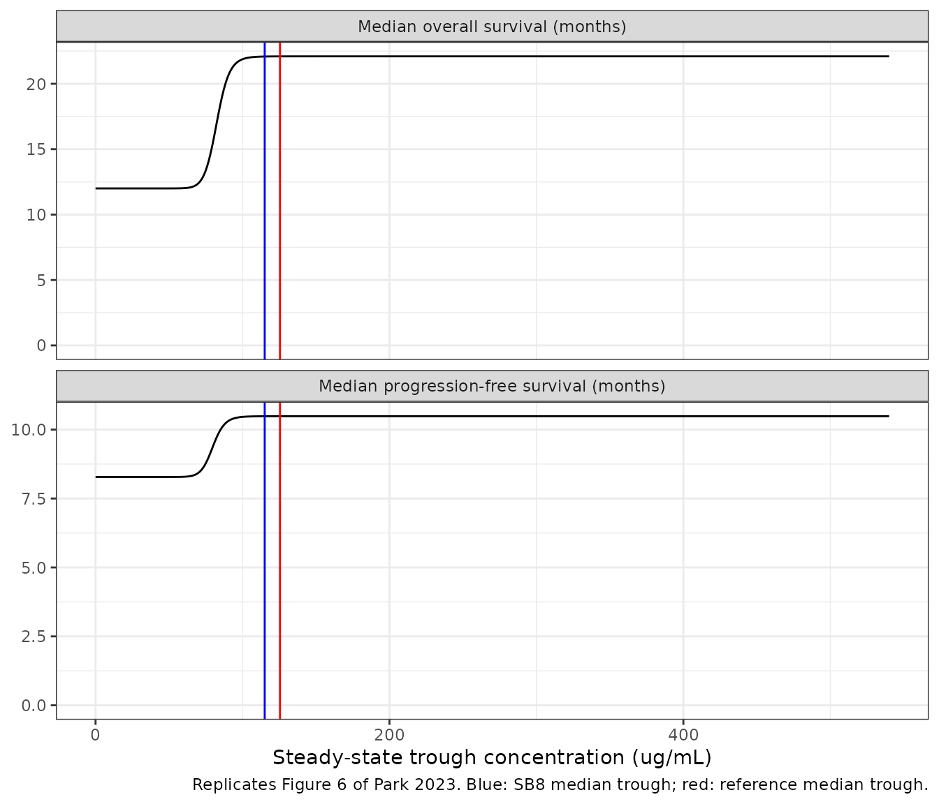
Virtual cohort and population survival curves
The visual predictive checks of Park 2023 (Figures 3-5) simulate the observed cohort with its own trough concentrations. The individual troughs are not published, so the cohort here takes the 224 troughs as evenly spaced quantiles of a log-normal distribution matched to the pooled median and interquartile range of Table 1 (119.5, 92.0-150.5 ug/mL). Using quantiles rather than random draws makes the cohort, and every check on it, deterministic. With the between-subject variance fixed at zero, the population survival curve is the mean of the individual survival curves.
n_cohort <- 224
trough_sdlog <- (log(150.5) - log(92.0)) / (2 * qnorm(0.75))
cohort <- data.frame(
  id = seq_len(n_cohort),
  CTROUGH = qlnorm(ppoints(n_cohort), meanlog = log(119.5), sdlog = trough_sdlog)
) |>
  mutate(quartile = paste0("Q", ntile(CTROUGH, 4)))
stopifnot(abs(median(cohort$CTROUGH) - 119.5) < 1)

cohort_events <- tidyr::expand_grid(id = cohort$id, time = seq(0, 24, by = 0.25)) |>
  left_join(cohort, by = "id") |>
  mutate(evid = 0, cmt = "cumhaz")

population_survival <- function(mod, endpoint) {
  rxode2::rxSolve(rxode2::zeroRe(mod), events = cohort_events, returnType = "data.frame") |>
    left_join(select(cohort, id, quartile), by = "id") |>
    mutate(endpoint = endpoint)
}
cohort_sim <- bind_rows(
  population_survival(mod_os, "Overall survival"),
  population_survival(mod_pfs, "Progression-free survival")
)
#> ℹ parameter labels from comments will be replaced by 'label()'
#> Warning: No sigma parameters in the model
#> ℹ omega/sigma items treated as zero: 'etallambda'
#> ℹ parameter labels from comments will be replaced by 'label()'
#> Warning: No sigma parameters in the model
#> ℹ omega/sigma items treated as zero: 'etallambda'
stopifnot(length(unique(cohort_sim$id)) == n_cohort)
# Replicates the model-predicted median curves of Figure 3 of Park 2023.
pop_curve <- cohort_sim |>
  group_by(endpoint, time) |>
  summarise(sur = mean(sur), .groups = "drop")

ggplot(pop_curve, aes(time, sur)) +
  geom_line(colour = "red") +
  geom_hline(yintercept = 0.5, linetype = "dotted") +
  facet_wrap(~endpoint, ncol = 1) +
  scale_x_continuous(breaks = seq(0, 24, by = 2)) +
  labs(
    x = "Time (months)",
    y = "Survival probability",
    caption = "Replicates the predicted median curves of Figure 3 of Park 2023."
  ) +
  theme_bw()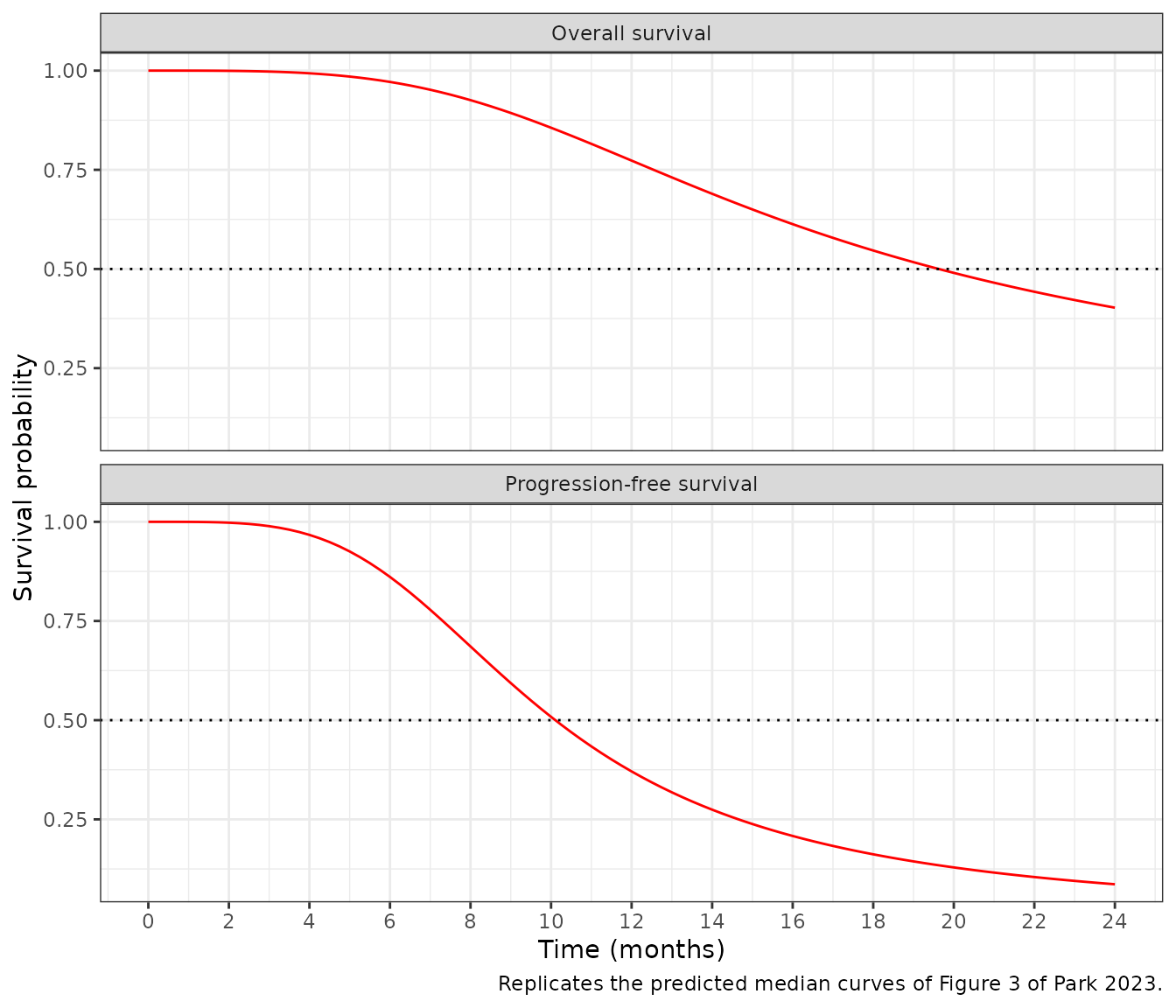
Figure 3 of Park 2023 shows the predicted median overall-survival curve crossing 0.5 at about 19.5-20 months and reaching about 0.40 at 24 months, and the progression-free curve crossing 0.5 at about 10 months and reaching about 0.08 at 24 months.
pop_median <- pop_curve |>
  group_by(endpoint) |>
  summarise(
    median_months = approx(sur, time, xout = 0.5, ties = mean)$y,
    sur_24 = sur[time == 24],
    .groups = "drop"
  )
pop_median
#> # A tibble: 2 × 3
#>   endpoint                  median_months sur_24
#>   <chr>                             <dbl>  <dbl>
#> 1 Overall survival                   19.6 0.402
#> 2 Progression-free survival          10.1 0.0864
stopifnot(nrow(pop_median) == 2)
os_row <- pop_median[pop_median$endpoint == "Overall survival", ]
pfs_row <- pop_median[pop_median$endpoint == "Progression-free survival", ]
# Figure 3 read-offs. The cohort is an approximation of the observed troughs
# (log-normal quantiles), so the bounds are sized for that, not for solver
# error.
stopifnot(
  abs(os_row$median_months - 19.75) < 1.5,
  abs(os_row$sur_24 - 0.40) < 0.05,
  abs(pfs_row$median_months - 10) < 1,
  abs(pfs_row$sur_24 - 0.08) < 0.04
)
# Replicates the model-predicted median curves of Figures 4 (OS) and 5 (PFS)
# of Park 2023: population survival stratified by trough-concentration
# quartile.
quartile_curve <- cohort_sim |>
  group_by(endpoint, quartile, time) |>
  summarise(sur = mean(sur), .groups = "drop")

ggplot(quartile_curve, aes(time, sur, colour = quartile)) +
  geom_line() +
  facet_wrap(~endpoint, ncol = 1) +
  scale_x_continuous(breaks = seq(0, 24, by = 2)) +
  labs(
    x = "Time (months)",
    y = "Survival probability",
    colour = "Trough quartile",
    caption = "Replicates the predicted median curves of Figures 4 and 5 of Park 2023."
  ) +
  theme_bw()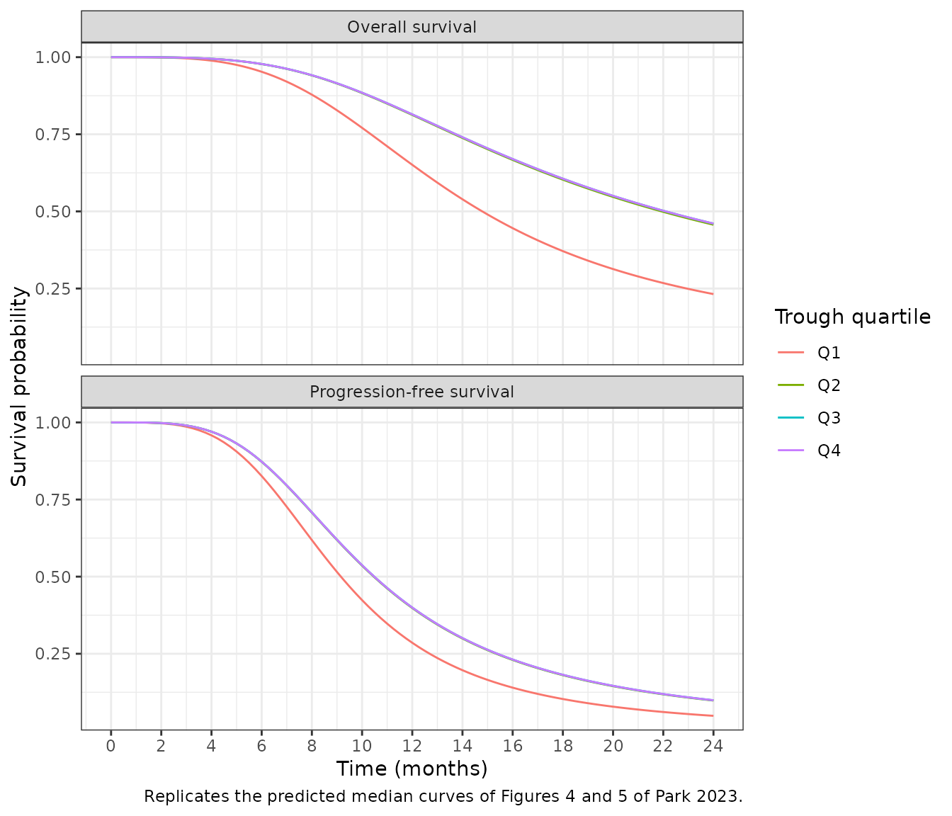
Only the lowest trough quartile, whose troughs straddle
ec50, has noticeably shorter survival; the upper three
quartiles sit on the plateau of the exposure-response curve.
PKNCA validation
Not applicable. The models contain no pharmacokinetics: the trough concentration is an input column and the outputs are a hazard, a survival probability and a median time to event, none of which is a concentration-time profile. The typical-value checks and the closed-form identity above take the place of the NCA comparison.
Assumptions and deviations
-
No between-subject variability. The control file
puts an exponential random effect on
lambda, but Table 3 reports no variance and the Discussion states that typical predictions were made.etallambdais carried atfixed(0). -
Progression-free survival structure. The
supplementary control file is the overall-survival one. Park 2023
Equations 3 and 4, the Results text and Table 3 give the same
log-logistic sigmoid-Emax structure for progression-free survival, so
Park_2023_bevacizumab_pfsuses the same equations with the Table 3 PFS estimates. -
Time unit. Table 3 does not print units for
lambda. Figures 3 and 6 are in months and the drug-free medians of Figure 6 (12 and about 8.3 months) equallambda, so time is in months. - The trough is time-fixed. One trough per patient, measured at steady state, applies from randomisation onward, including the induction cycles before steady state. A user simulating a new regimen should supply that regimen’s steady-state trough, not a time-varying concentration.
- Virtual cohort. The troughs of the 224 patients are not published. The population curves above use log-normal quantiles matched to the Table 1 median and interquartile range, which is why the Figure 3 comparison has read-off-sized rather than solver-sized tolerances.
- Maximum medians. Park 2023 prints the 50% and 90% medians and concentrations but not the maximum median itself; 22.2 and 10.5 months are read from the plateaus of Figure 6.