Tacrolimus plasma and whole blood (Koomen 2023)
Source:vignettes/articles/Koomen_2023_tacrolimus.Rmd
Koomen_2023_tacrolimus.RmdModel and source
- Citation: Koomen JV, Knobbe TJ, Zijp TR, Kremer D, Gan CT, Verschuuren EAM, Bakker SJL, Touw DJ, Colin PJ; TransplantLines Investigators. A Joint Pharmacokinetic Model for the Simultaneous Description of Plasma and Whole Blood Tacrolimus Concentrations in Kidney and Lung Transplant Recipients. Clin Pharmacokinet. 2023;62(8):1117. doi:10.1007/s40262-023-01259-x
- Description: Joint one-compartment population PK model for plasma (Cc) and whole-blood (Cblood) tacrolimus trough concentrations in adult kidney and lung transplant recipients (Koomen 2023). Plasma is described by first-order absorption (ka and F fixed) and first-order elimination; whole blood is the haematocrit-weighted sum of the plasma concentration and an erythrocyte-bound concentration that saturates in plasma (Bmax, Kd). Bioavailability depends on daily dose (per formulation: Prograf, Advagraf, Envarsus), food intake and time after transplantation (Prograf only); apparent CL on haematocrit, eGFR and transplant type; V on haptoglobin; Bmax on haematocrit, total cholesterol, haptoglobin, vitamin B12, transplant type and concomitant mycophenolic acid and vitamin D3.
- Article: https://doi.org/10.1007/s40262-023-01259-x (open access; the electronic supplementary material holds the covariate screen, the base-model estimates and the covariate-effect simulations ESM Figs 1 and 2)
Koomen 2023 fitted plasma and whole-blood tacrolimus trough concentrations jointly. Plasma follows a one-compartment model with first-order absorption (Eq. 1). Whole blood is the haematocrit-weighted sum of the plasma concentration and an erythrocyte-bound concentration that saturates in plasma (Eqs. 2 and 4):
Cblood = Cc * (1 - HCT/100) + Cbound * HCT/100Cbound = Cc * Bmax / (Kd + Cc)
with Bmax the maximum bound concentration and
Kd the plasma concentration at half-maximal binding (Table
2 calls it C50). The two concentrations are assumed to be
in equilibrium at sampling.
Population
The model was developed in 1060 adult transplant recipients of the TransplantLines Biobank and Cohort Study (University Medical Center Groningen, the Netherlands): 845 kidney and 215 lung recipients (Table 1). Mean (SD) age was 54.7 (13.6) years, body weight 81.0 (16.3) kg, eGFR 50.2 (19.2) mL/min/1.73 m^2 and haematocrit 39.0 (5.5)%; 39.5% were female and 91.0% Caucasian. The first sample was taken a median of 47 days (range 2-409) after transplantation. Tacrolimus was titrated by whole-blood therapeutic drug monitoring: Prograf twice daily (74.7% of plasma samples), Advagraf once daily (18.5%) or Envarsus once daily (5.4%). The data comprised 1973 plasma and 1961 whole-blood trough concentrations (2.5 samples per patient on average), drawn at 08:00 after an overnight fast, which places the sample 10 h after the last dose of a twice-daily regimen and 22 h after a once-daily dose.
The same information is available programmatically via
readModelDb("Koomen_2023_tacrolimus")()$population.
Source trace
Every ini() value carries an in-file comment pointing to
its source. The table collects them.
| Equation / parameter | Value | Source location |
|---|---|---|
lka (fixed) |
log(3.5) 1/h | Methods, Eq. 5 |
lfdepot (fixed) |
log(0.25) | Methods, Eq. 8 |
lcl |
log(257.6) L/h | Table 2, Eq. 6 |
lvc |
log(4213.2) L | Table 2, Eq. 7 |
lbmax |
log(35.7) ng/mL | Table 2, Eq. 9 |
lkd |
log(0.24) ng/mL | Table 2 (C50), Eq. 10 |
e_dose_tac_fdepot_prograf / _advagraf /
_envarsus
|
-0.64 / -0.62 / -0.74 | Table 2, Eq. 8 |
e_pod_fdepot |
-0.32 | Table 2, Eq. 8 |
e_fasted_fdepot |
-0.11 | Table 2, Eq. 8 |
e_hct_cl, e_crcl_cl,
e_tx_lung_cl
|
0.49, 0.07, -0.22 | Table 2, Eq. 6 |
e_haptoglobin_vc |
0.13 | Table 2, Eq. 7 |
e_hct_bmax, e_tchol_bmax,
e_haptoglobin_bmax, e_vitamin_b12_bmax
|
-0.43, -0.18, -0.05, 0.04 | Table 2, Eq. 9 |
e_tx_lung_bmax, e_conmed_mpa_bmax,
e_conmed_colecalciferol_bmax
|
0.10, 0.14, 0.05 | Table 2, Eq. 9 |
etalfdepot + etalbmax |
0.13, -0.02, 0.02 | Table 2 (BSV F, BSV Bmax, covariance) |
propSd |
0.371 | Table 2 (plasma, CV 37.1%) |
propSd_Cblood |
0.253 | Table 2 (whole blood, CV 25.3%) |
d/dt(depot), d/dt(central)
|
– | Eq. 1 (ADVAN2/TRANS2) |
Cblood, Cbound
|
– | Eqs. 2 and 4 |
| Covariate reference values | Dose 2.5 mg/day, HCT 39%, eGFR 51, haptoglobin 1.4 g/L, cholesterol 4.6 mmol/L, vitamin B12 320 pmol/L | Eqs. 6-9 |
Reference subject and marginal covariate effects (ESM Figs 1 and 2)
ESM Figs 1 and 2 show the median and 95% prediction interval of the plasma and whole-blood trough for a reference subject and for one-at-a-time covariate changes, at month 6 and month 3 after transplantation. The reference subject is a kidney recipient on 3 mg/day Prograf, fasted, with haematocrit 39%, eGFR 50 mL/min/1.73 m^2, haptoglobin 1.5 g/L, total cholesterol 4.8 mmol/L, vitamin B12 400 pmol/L, mycophenolic acid and no vitamin D3 (ESM figure captions).
Each scenario is simulated at steady state, sampled at the trough
time the paper assumed (10 h after a twice-daily dose, 22 h after a
once-daily dose), both as the typical value and as 200 subjects with
between-subject variability on F and Bmax. The paper’s prediction
intervals come from between-subject variability alone: the reference
interval 0.05-0.19 ng/mL is the typical 0.09 times
exp(+/-1.96 * sqrt(0.13)), with no residual error.
mod <- readModelDb("Koomen_2023_tacrolimus")
mod_typ <- rxode2::zeroRe(mod)
#> ℹ parameter labels from comments will be replaced by 'label()'

ref_cov <- tibble(
  DOSE_TAC_MGD = 3, FORM_TAC_IR = 1, FORM_TAC_ENVARSUS = 0, FED = 0,
  HCT = 39, CRCL = 50, TX_LUNG = 0, HAPTOGLOBIN = 1.5, TCHOL = 4.8,
  VITAMIN_B12 = 400, CONMED_MPA = 1, CONMED_COLECALCIFEROL = 0
)

scenario_changes <- list(
  "Reference" = list(),
  "Dose 0.5 mg" = list(DOSE_TAC_MGD = 0.5),
  "Dose 25 mg" = list(DOSE_TAC_MGD = 25),
  "Advagraf" = list(FORM_TAC_IR = 0),
  "Envarsus" = list(FORM_TAC_IR = 0, FORM_TAC_ENVARSUS = 1),
  "Fed" = list(FED = 1),
  "Lung" = list(TX_LUNG = 1),
  "Total cholesterol 2.0 mmol/L" = list(TCHOL = 2),
  "Total cholesterol 7.0 mmol/L" = list(TCHOL = 7),
  "eGFR 10 mL/min/1.73 m2" = list(CRCL = 10),
  "eGFR 120 mL/min/1.73 m2" = list(CRCL = 120),
  "Haptoglobin 0.5 g/L" = list(HAPTOGLOBIN = 0.5),
  "Haptoglobin 3.0 g/L" = list(HAPTOGLOBIN = 3),
  "Haematocrit 20%" = list(HCT = 20),
  "Haematocrit 60%" = list(HCT = 60),
  "No mycophenolic acid" = list(CONMED_MPA = 0),
  "Vitamin B12 100 pmol/L" = list(VITAMIN_B12 = 100),
  "Vitamin B12 1000 pmol/L" = list(VITAMIN_B12 = 1000),
  "Vitamin D3" = list(CONMED_COLECALCIFEROL = 1)
)
months <- c("Month 3" = 91.25, "Month 6" = 182.5)

# One steady-state dose and one trough observation per subject. The daily dose
# is split over two administrations for Prograf; DOSE_TAC_MGD stays the daily
# total because Eq. 8 normalises it to 2.5 mg/day.
make_scenario <- function(scenario, month, n, id_offset) {
  cv <- ref_cov
  for (k in names(scenario_changes[[scenario]])) {
    cv[[k]] <- scenario_changes[[scenario]][[k]]
  }
  once_daily <- cv$FORM_TAC_IR == 0
  tau <- if (once_daily) 24 else 12
  subj <- cv[rep(1, n), ] |>
    mutate(
      id = id_offset + seq_len(n),
      POD = months[[month]],
      scenario = scenario,
      month = month
    )
  bind_rows(
    subj |> mutate(time = 0, amt = DOSE_TAC_MGD * tau / 24, ii = tau, ss = 1L,
                   evid = 1L, cmt = "depot", dvid = NA_integer_),
    subj |> mutate(time = if (once_daily) 22 else 10, amt = 0, ii = 0, ss = 0L,
                   evid = 0L, cmt = "central", dvid = 1L)
  ) |>
    arrange(id, time, desc(evid))
}

grid <- expand_grid(scenario = names(scenario_changes), month = names(months))
build <- function(n) {
  bind_rows(lapply(seq_len(nrow(grid)), function(i) {
    make_scenario(grid$scenario[i], grid$month[i], n, id_offset = (i - 1L) * n)
  }))
}
ev_typ <- build(1L)
ev_iiv <- build(200L)
stopifnot(!anyDuplicated(unique(ev_iiv[, c("id", "time", "evid")])))

keep_cols <- c("scenario", "month")
sim_typ <- rxode2::rxSolve(mod_typ, events = ev_typ, keep = keep_cols,
                           returnType = "data.frame")
#> ℹ omega/sigma items treated as zero: 'etalfdepot', 'etalbmax'
#> Warning: multi-subject simulation without without 'omega'
rxode2::rxSetSeed(20230601)
sim_iiv <- rxode2::rxSolve(mod, events = ev_iiv, keep = keep_cols,
                           returnType = "data.frame")
#> ℹ parameter labels from comments will be replaced by 'label()'
# Residual error is not part of the published intervals: use the individual
# predictions (Cc and Cblood are the error-free model values in the output).
stopifnot(!anyNA(sim_typ$Cc), !anyNA(sim_iiv$Cc), !anyNA(sim_iiv$Cblood))

forest <- sim_iiv |>
  pivot_longer(c(Cc, Cblood), names_to = "matrix", values_to = "conc") |>
  group_by(scenario, month, matrix) |>
  summarise(med = median(conc), lo = quantile(conc, 0.025),
            hi = quantile(conc, 0.975), .groups = "drop") |>
  mutate(scenario = factor(scenario, levels = rev(names(scenario_changes))),
         matrix = factor(ifelse(matrix == "Cc", "Plasma", "Whole blood"),
                         levels = c("Plasma", "Whole blood")))
ggplot(forest, aes(med, scenario)) +
  geom_errorbar(aes(xmin = lo, xmax = hi), width = 0.3, orientation = "y") +
  geom_point(shape = 15) +
  facet_grid(month ~ matrix, scales = "free_x") +
  scale_x_log10() +
  labs(x = "Tacrolimus trough concentration (ng/mL)", y = NULL,
       caption = paste("Replicates ESM Figs 1 (month 6) and 2 (month 3) of",
                       "Koomen 2023: median and 95% prediction interval,",
                       "200 simulated subjects per scenario."))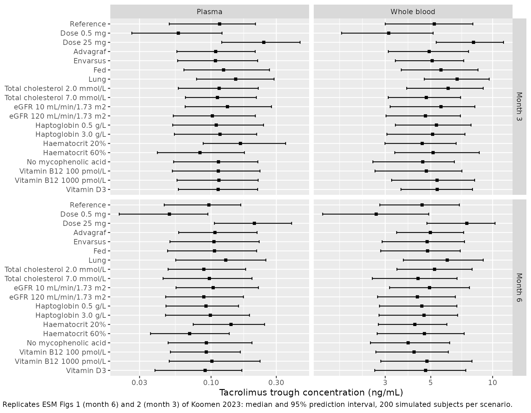
Comparison with the reported values
The Results (“Simulations”) quote the month-6 medians and 95% prediction intervals for the reference subject and for the dose and haematocrit extremes. The paper reports plasma to 0.01 ng/mL and whole blood to 0.1 ng/mL.
published <- tribble(
  ~scenario, ~pub_cc, ~pub_cc_lo, ~pub_cc_hi, ~pub_cb, ~pub_cb_lo, ~pub_cb_hi,
  "Reference", 0.09, 0.05, 0.19, 4.4, 2.7, 7.0,
  "Dose 0.5 mg", 0.05, 0.02, 0.10, 2.7, 1.6, 4.6,
  "Dose 25 mg", 0.20, 0.10, 0.41, 7.2, 4.9, 10.6,
  "Haematocrit 20%", 0.14, 0.07, 0.29, 4.1, 2.7, 6.3,
  "Haematocrit 60%", 0.07, 0.04, 0.14, 4.5, 2.7, 7.4
)

typ6 <- sim_typ |>
  filter(month == "Month 6") |>
  select(scenario, typ_cc = Cc, typ_cb = Cblood)
pi6 <- forest |>
  filter(month == "Month 6") |>
  mutate(scenario = as.character(scenario)) |>
  select(scenario, matrix, med, lo, hi) |>
  pivot_wider(names_from = matrix, values_from = c(med, lo, hi))

cmp <- published |>
  left_join(typ6, by = "scenario") |>
  left_join(pi6, by = "scenario")

cmp |>
  transmute(
    scenario,
    plasma_pub = sprintf("%.2f (%.2f-%.2f)", pub_cc, pub_cc_lo, pub_cc_hi),
    plasma_typ = sprintf("%.3f", typ_cc),
    plasma_sim = sprintf("%.3f (%.3f-%.3f)", med_Plasma, lo_Plasma, hi_Plasma),
    wb_pub = sprintf("%.1f (%.1f-%.1f)", pub_cb, pub_cb_lo, pub_cb_hi),
    wb_typ = sprintf("%.2f", typ_cb),
    wb_sim = sprintf("%.2f (%.2f-%.2f)", `med_Whole blood`,
                     `lo_Whole blood`, `hi_Whole blood`)
  ) |>
  rename(
    "Scenario (month 6)" = scenario,
    "Plasma, published" = plasma_pub,
    "Plasma, typical" = plasma_typ,
    "Plasma, simulated median (95% PI)" = plasma_sim,
    "Whole blood, published" = wb_pub,
    "Whole blood, typical" = wb_typ,
    "Whole blood, simulated median (95% PI)" = wb_sim
  ) |>
  knitr::kable(caption = paste("Month-6 trough concentrations (ng/mL):",
"Koomen 2023 Results versus the packaged model."))| Scenario (month 6) | Plasma, published | Plasma, typical | Plasma, simulated median (95% PI) | Whole blood, published | Whole blood, typical | Whole blood, simulated median (95% PI) |
|---|---|---|---|---|---|---|
| Reference | 0.09 (0.05-0.19) | 0.094 | 0.096 (0.045-0.165) | 4.4 (2.7-7.0) | 4.50 | 4.54 (2.82-6.89) |
| Dose 0.5 mg | 0.05 (0.02-0.10) | 0.049 | 0.050 (0.021-0.095) | 2.7 (1.6-4.6) | 2.72 | 2.71 (1.49-4.89) |
| Dose 25 mg | 0.20 (0.10-0.41) | 0.201 | 0.207 (0.106-0.388) | 7.2 (4.9-10.6) | 7.34 | 7.49 (4.79-10.28) |
| Haematocrit 20% | 0.14 (0.07-0.29) | 0.140 | 0.140 (0.074-0.246) | 4.1 (2.7-6.3) | 4.10 | 4.18 (2.78-5.99) |
| Haematocrit 60% | 0.07 (0.04-0.14) | 0.071 | 0.070 (0.036-0.136) | 4.5 (2.7-7.4) | 4.66 | 4.66 (2.74-7.27) |
# Typical values are deterministic (same parameters, no random draw), so the
# check is tight: plasma within the 0.01 ng/mL rounding of the paper plus a
# small margin, whole blood within 6%. A mis-transcribed CL, V, Bmax, Kd or
# covariate exponent moves at least one of these rows by far more.
stopifnot(
  all(abs(cmp$typ_cc - cmp$pub_cc) < 0.006),
  all(abs(cmp$typ_cb / cmp$pub_cb - 1) < 0.06)
)
The typical values match the reported medians within their rounding. The simulated intervals come from 200 subjects per scenario, so their tails move by several percent between renders; they agree with the published intervals to about that precision.
Time after transplantation is in hours
Table 2 labels the time-after-transplantation covariate in days, and
Eq. 8 divides it by 1000. With time in days the Prograf term
1 + exp(-0.32 * time / 1000) changes by only 1.5% between
month 3 and month 6, whereas ESM Figs 1 and 2 show the reference plasma
trough falling from about 0.115 ng/mL (month 3, digitised by the
maintainers) to 0.093 ng/mL (month 6), a 1.2-fold drop. Only time in
hours reproduces that drop, so the model converts POD
(days) to hours before applying the published coefficient.
ratio_hours <- with(
  sim_typ |> filter(scenario == "Reference"),
  Cc[month == "Month 3"] / Cc[month == "Month 6"]
)
time_term <- function(t) 1 + exp(-0.32 * t / 1000)
ratio_days <- time_term(91.25) / time_term(182.5)
tibble(
  reading = c("Time in hours (packaged model)", "Time in days", "ESM Figs 1-2 (digitised)"),
  "Month 3 / month 6 plasma trough" = c(ratio_hours, ratio_days, 0.115 / 0.093)
) |>
knitr::kable(digits = 3)| reading | Month 3 / month 6 plasma trough |
|---|---|
| Time in hours (packaged model) | 1.201 |
| Time in days | 1.014 |
| ESM Figs 1-2 (digitised) | 1.237 |
Plasma-whole blood relationship and plasma target ranges (Fig. 3)
Fig. 3 maps plasma trough concentrations onto whole-blood concentrations using each patient’s covariates and the between-subject variability on Bmax, and translates the whole-blood target ranges into plasma ranges. The original covariates are not public, so a virtual cohort of 200 kidney and 200 lung recipients is drawn from the Table 1 means and SDs.
set.seed(2023)
draw_lognormal <- function(n, m, s) {
  sg <- sqrt(log(1 + (s / m)^2))
  rlnorm(n, log(m) - sg^2 / 2, sg)
}
make_cohort <- function(n, lung, hct, tchol, hapto, b12, p_mpa, p_vitd,
                        id_offset) {
  tibble(
    id = id_offset + seq_len(n),
    TX_LUNG = lung,
    HCT = pmin(pmax(rnorm(n, hct[1], hct[2]), 20), 60),
    TCHOL = pmax(rnorm(n, tchol[1], tchol[2]), 2),
    HAPTOGLOBIN = pmax(rnorm(n, hapto[1], hapto[2]), 0.1),
    VITAMIN_B12 = draw_lognormal(n, b12[1], b12[2]),
    CONMED_MPA = rbinom(n, 1, p_mpa),
    CONMED_COLECALCIFEROL = rbinom(n, 1, p_vitd)
  )
}
cohort <- bind_rows(
  make_cohort(200, 0, c(39.5, 5.6), c(4.7, 1.1), c(1.5, 0.7), c(380.7, 232.3),
              0.839, 0.399, id_offset = 0L),
  make_cohort(200, 1, c(37.2, 4.6), c(4.9, 1.3), c(1.4, 0.7), c(476.0, 322.9),
              0.828, 0.372, id_offset = 200L)
) |>
  mutate(DOSE_TAC_MGD = 3, FORM_TAC_IR = 1, FORM_TAC_ENVARSUS = 0, FED = 0,
         POD = 182.5, CRCL = 50)

ev_cohort <- bind_rows(
  cohort |> mutate(time = 0, amt = 1.5, ii = 12, ss = 1L, evid = 1L,
                   cmt = "depot", dvid = NA_integer_),
  cohort |> mutate(time = 10, amt = 0, ii = 0, ss = 0L, evid = 0L,
                   cmt = "central", dvid = 1L)
) |>
  arrange(id, time, desc(evid))
stopifnot(!anyDuplicated(unique(ev_cohort[, c("id", "time", "evid")])))

rxode2::rxSetSeed(20230602)
sim_cohort <- rxode2::rxSolve(mod, events = ev_cohort, keep = c("TX_LUNG", "HCT"),
                              returnType = "data.frame")
binding <- sim_cohort |>
  select(id, TX_LUNG, HCT, bmax, kd) |>
  distinct(id, .keep_all = TRUE)
stopifnot(nrow(binding) == 400, !anyNA(binding$bmax))
For each simulated patient the whole-blood concentration at a given
plasma concentration follows directly from Eqs. 2 and 4 with that
patient’s bmax and kd; residual error is not
added, matching the paper’s prediction intervals.
plasma_grid <- seq(0, 2, by = 0.01)
relation <- expand_grid(binding, Cc = plasma_grid) |>
  mutate(
    Cblood = Cc * (1 - HCT / 100) + Cc * bmax / (kd + Cc) * HCT / 100,
    recipient = ifelse(TX_LUNG == 1, "Lung", "Kidney")
  )

targets <- tribble(
  ~recipient, ~range, ~lo, ~hi,
  "Kidney", "6-10 ng/mL (month 3)", 6, 10,
  "Kidney", "4-6 ng/mL (month 6 and later)", 4, 6,
  "Lung", "7-10 ng/mL (month 3 and later)", 7, 10
)

relation |>
  filter(Cc <= 0.5) |>
  group_by(recipient, Cc) |>
  summarise(lo = quantile(Cblood, 0.025), med = median(Cblood),
            hi = quantile(Cblood, 0.975), .groups = "drop") |>
  ggplot(aes(Cc, med)) +
  geom_ribbon(aes(ymin = lo, ymax = hi), alpha = 0.25) +
  geom_line() +
  geom_hline(data = targets, aes(yintercept = lo, linetype = range)) +
  geom_hline(data = targets, aes(yintercept = hi, linetype = range)) +
  facet_wrap(~recipient) +
  labs(x = "Plasma tacrolimus (ng/mL)", y = "Whole-blood tacrolimus (ng/mL)",
       linetype = "Whole-blood target",
       caption = paste("Replicates Fig. 3a-b of Koomen 2023: median and 95%",
                       "prediction interval of whole blood versus plasma."))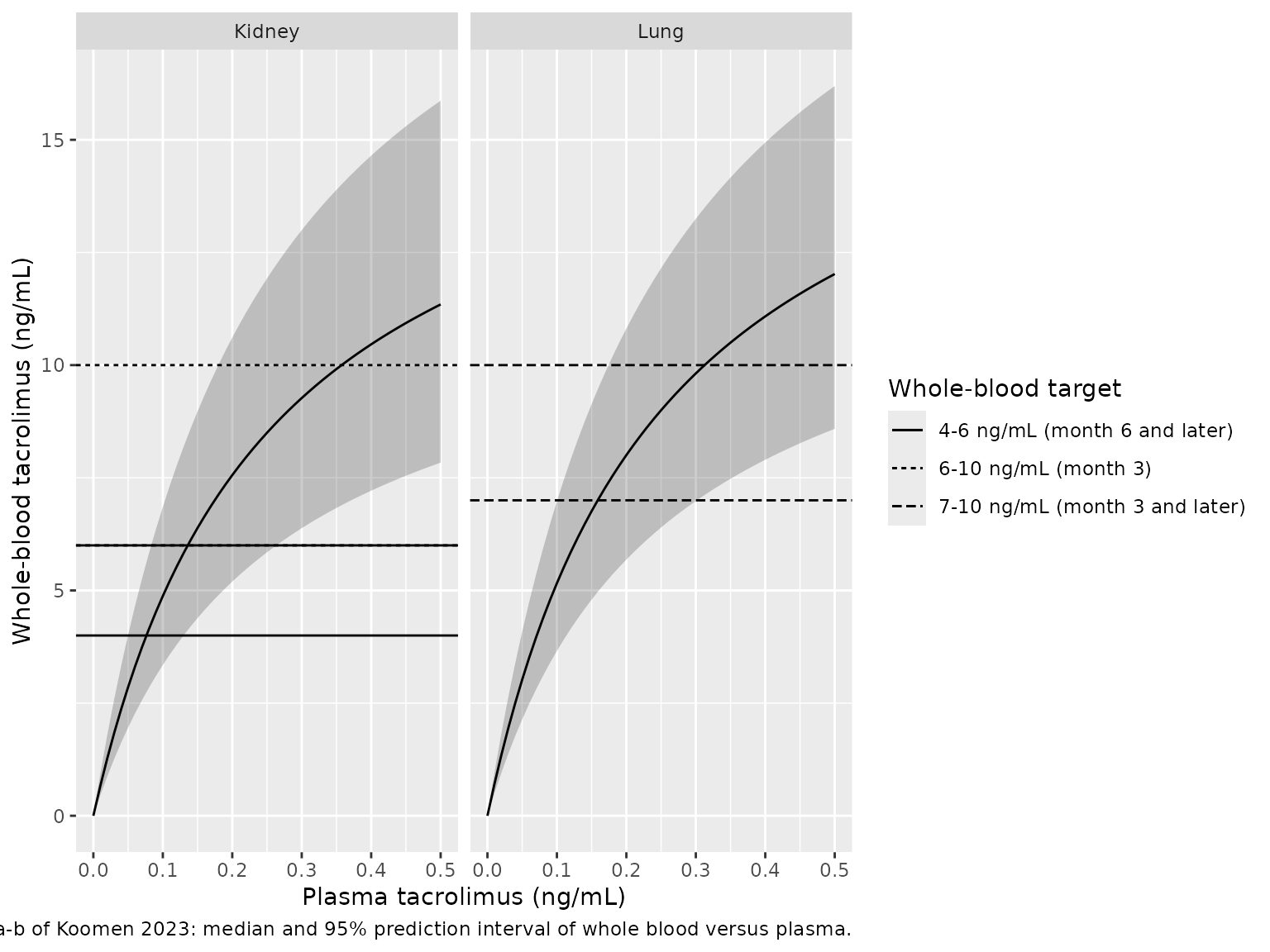
plasma_ranges <- targets |>
  rowwise() |>
  mutate(
    sel = list(relation$Cc[relation$recipient == recipient &
                             relation$Cblood >= lo & relation$Cblood <= hi]),
    sim_lo = quantile(sel, 0.025),
    sim_hi = quantile(sel, 0.975)
  ) |>
  ungroup() |>
  mutate(published = c("0.10-1.18", "0.06-0.26", "0.10-0.93"))

plasma_ranges |>
  transmute(recipient, range,
            simulated = sprintf("%.2f-%.2f", sim_lo, sim_hi), published) |>
  rename(
    "Recipient" = recipient,
    "Whole-blood target" = range,
    "Plasma range, virtual cohort (ng/mL)" = simulated,
    "Plasma range, Koomen 2023 (ng/mL)" = published
  ) |>
  knitr::kable(caption = paste("95% range of plasma concentrations whose",
                               "predicted whole-blood concentration lies in",
"the target range."))| Recipient | Whole-blood target | Plasma range, virtual cohort (ng/mL) | Plasma range, Koomen 2023 (ng/mL) |
|---|---|---|---|
| Kidney | 6-10 ng/mL (month 3) | 0.12-1.20 | 0.10-1.18 |
| Kidney | 4-6 ng/mL (month 6 and later) | 0.06-0.24 | 0.06-0.26 |
| Lung | 7-10 ng/mL (month 3 and later) | 0.14-0.75 | 0.10-0.93 |
The kidney ranges from the virtual cohort agree closely with the published ones. The lung range comes out narrower than the published 0.10-0.93 ng/mL, mostly at its upper end. The paper used the observed covariates of all 1060 patients, whose joint distribution (for example the correlation of haematocrit with cholesterol and haptoglobin) a cohort drawn from independent marginal summaries does not carry. The ranges are therefore shown for comparison and are not used as a gate.
PKNCA: steady-state exposure of the reference subject
The paper reports troughs only and no NCA. As an internal check,
PKNCA computes the steady-state average, minimum and maximum plasma
concentration of the typical reference subject (3 mg/day, month 6) for
each formulation over one dosing interval. Under linear kinetics the
average must equal F * dose / (CL * tau) with the subject’s
own F and CL.
form_cov <- list(
  Prograf = list(FORM_TAC_IR = 1, FORM_TAC_ENVARSUS = 0, tau = 12),
  Advagraf = list(FORM_TAC_IR = 0, FORM_TAC_ENVARSUS = 0, tau = 24),
  Envarsus = list(FORM_TAC_IR = 0, FORM_TAC_ENVARSUS = 1, tau = 24)
)
ev_nca <- bind_rows(lapply(seq_along(form_cov), function(i) {
  f <- form_cov[[i]]
  subj <- ref_cov |>
    mutate(id = i, POD = 182.5, treatment = names(form_cov)[i],
           FORM_TAC_IR = f$FORM_TAC_IR, FORM_TAC_ENVARSUS = f$FORM_TAC_ENVARSUS)
  bind_rows(
    subj |> mutate(time = 0, amt = DOSE_TAC_MGD * f$tau / 24, ii = f$tau,
                   ss = 1L, evid = 1L, cmt = "depot", dvid = NA_integer_),
    subj[rep(1, f$tau * 10 + 1), ] |>
      mutate(time = seq(0, f$tau, by = 0.1), amt = 0, ii = 0, ss = 0L,
             evid = 0L, cmt = "central", dvid = 1L)
  )
})) |>
  arrange(id, time, desc(evid))

sim_nca <- rxode2::rxSolve(mod_typ, events = ev_nca, keep = "treatment",
                           returnType = "data.frame")
#> ℹ omega/sigma items treated as zero: 'etalfdepot', 'etalbmax'
#> Warning: multi-subject simulation without without 'omega'
stopifnot(!anyNA(sim_nca$Cc))

conc_df <- sim_nca |>
  filter(!is.na(Cc)) |>
  select(id, time, Cc, treatment)
dose_df <- ev_nca |>
  filter(evid == 1) |>
  select(id, time, amt, treatment)
tau_df <- tibble(treatment = names(form_cov),
                 tau = vapply(form_cov, function(f) f$tau, numeric(1)))

conc_obj <- PKNCA::PKNCAconc(conc_df, Cc ~ time | treatment + id)
dose_obj <- PKNCA::PKNCAdose(dose_df, amt ~ time | treatment + id)
intervals <- tau_df |>
  transmute(treatment, start = 0, end = tau, cmax = TRUE, cmin = TRUE,
            cav = TRUE) |>
  as.data.frame()
nca_res <- PKNCA::pk.nca(PKNCA::PKNCAdata(conc_obj, dose_obj,
                                          intervals = intervals))

nca_tab <- as.data.frame(nca_res) |>
  select(treatment, PPTESTCD, PPORRES) |>
  pivot_wider(names_from = PPTESTCD, values_from = PPORRES)

closed_form <- sim_nca |>
  group_by(treatment) |>
  slice(1) |>
  ungroup() |>
  left_join(tau_df, by = "treatment") |>
  mutate(cav_expected = 1000 * fdepot * ref_cov$DOSE_TAC_MGD * tau / 24 /
           (cl * tau)) |>
  select(treatment, cav_expected)

nca_check <- left_join(nca_tab, closed_form, by = "treatment")
nca_check |>
  rename(
    "Formulation" = treatment,
    "AUC0-tau (ng*h/mL)" = auclast,
    "Cmax (ng/mL)" = cmax,
    "Cmin (ng/mL)" = cmin,
    "Cav, PKNCA (ng/mL)" = cav,
    "Cav, F x dose / (CL x tau) (ng/mL)" = cav_expected
  ) |>
  knitr::kable(digits = 4, caption = paste("Steady-state plasma exposure of",
"the typical reference subject."))| Formulation | AUC0-tau (ng*h/mL) | Cmax (ng/mL) | Cmin (ng/mL) | Cav, PKNCA (ng/mL) | Cav, F x dose / (CL x tau) (ng/mL) |
|---|---|---|---|---|---|
| Prograf | 1.4385 | 0.1589 | 0.0830 | 0.1199 | 0.1199 |
| Advagraf | 5.2069 | 0.3849 | 0.0980 | 0.2170 | 0.2170 |
| Envarsus | 5.0942 | 0.3765 | 0.0959 | 0.2123 | 0.2123 |
Assumptions and deviations
-
Dose is the daily dose. Eq. 8 writes the
bioavailability covariate as
Dose / 2.5without saying whetherDoseis the daily or the per-administration amount. The daily-dose reading reproduces the paper’s own reference-subject simulations (3 mg Prograf -> 0.09 ng/mL plasma, 4.4 ng/mL whole blood); a per-administration reading gives 0.15-0.19 ng/mL. The model takesDOSE_TAC_MGDin mg/day, and a twice-daily regimen gives half of it per administration. -
Time after transplantation in hours. See the
section above: Table 2 labels the covariate in days, but only hours
reproduce ESM Figs 1 and 2. The model accepts
PODin days and converts it. - Food effect in ESM Fig. 1. The model applies the 11% lower F when fasted to Prograf only, as Eq. 8 prints it. In ESM Fig. 1 the “Fed”, “Advagraf” and “Envarsus” scenarios all lie about 11% below what Eq. 8 gives (digitised by the maintainers: about 0.094, 0.098 and 0.096 ng/mL against 0.105, 0.111 and 0.108 ng/mL here), which matches the fasted factor being applied in every scenario of that figure. The printed equation and the Table 2 label (“Prograft, fasted”) were followed. The ESM figure panels are therefore replicated in shape but are not used as a gate.
-
Vitamin D term. Eq. 9 is typeset as
1 x 0.05 + VitaminD; the model uses1 + 0.05 * CONMED_COLECALCIFEROL, the “Proportional” structure Table 2 lists for this effect. -
Fed indicator orientation. The paper codes
fasted(1 = fasted). The model uses the register columnFED(1 = fed), withfasted = 1 - FED. -
Formulation coding. Prograf, Advagraf and Envarsus
are encoded by
FORM_TAC_IR(Prograf) andFORM_TAC_ENVARSUS; Advagraf is the level with both indicators 0. The time-after-transplantation and food terms apply to Prograf only (Eq. 8); for the once-daily products the time term evaluates to1 + exp(0) = 2as printed. - Residual error. Both matrices have proportional error. Table 2 gives variances 0.14 and 0.06 with CV 37.1% and 25.3% (CV = sqrt(variance), per the table footnote); the CVs carry more digits and are used. The Results text quotes 37.3% for plasma, which is the CV of the between-subject variability on F; Table 2 is followed. The covariance between the plasma and whole-blood residuals (0.06, r = 0.60, estimated with the NONMEM L2 data item) cannot be expressed in the model’s residual-error syntax and is not encoded, so simulations that add residual error draw the two matrices independently.
- Between-subject variability. Only F and Bmax carry random effects; the variances 0.13 and 0.02 and covariance -0.02 are taken as printed. The printed CV for Bmax (14.4%) implies a variance of 0.0205, so 0.02 is a rounded value.
-
Haematocrit units.
HCTis in percent for the power effects (reference 39%) and used as the fractionHCT / 100in the whole-blood equation. -
New covariate columns.
HAPTOGLOBIN(g/L) andVITAMIN_B12(pmol/L) were added to the covariate register for this model, with spelled-out names ratified by the maintainers.CONMED_MPAandCONMED_COLECALCIFEROLfollow theCONMED_<INN>family. - Not reproduced. The prediction-corrected VPCs of Fig. 2 need the observed data, which are not public. Fig. 3c-d (percentage of patients in the whole-blood target range by plasma concentration) is summarised by the plasma-range table rather than redrawn.
- Errata. No correction notice is linked to this article in Europe PMC or PubMed as of 2026-11-06.