Telisotuzumab vedotin conjugate, MMAE payload and exposure-response (Babel 2026)
Source:vignettes/articles/Babel_2026_telisotuzumab.Rmd
Babel_2026_telisotuzumab.RmdSource and models
- Citation: Babel H, Brunsdon P, Engelhardt B, Schmitt V, Ratajczak C, Mensing S, Menon RM, Parikh A. Population pharmacokinetics and exposure-response analyses for telisotuzumab vedotin in patients with c-Met protein overexpressing tumors. CPT Pharmacometrics Syst Pharmacol. 2026;15(1):e70219. doi:10.1002/psp4.70219. PMCID PMC12945708. All parameter values are from Data S1 (Supporting Information) Table S7, ‘Final Model Parameter Estimates and Variability of Teliso-V Conjugate and Unconjugated MMAE Payload Pharmacokinetics’, Teliso-V Conjugate block.
- Article (open access): https://doi.org/10.1002/psp4.70219
- PubMed Central: https://www.ncbi.nlm.nih.gov/pmc/articles/PMC12945708/
- Supporting Information (Data S1; Tables S1-S7 and Figures S1-S5): distributed with the open-access article (PMC12945708).
Babel 2026 reports six models, and this package carries all six as separate files because the authors fitted them separately:
| Model file | What it is | Source |
|---|---|---|
Babel_2026_telisotuzumab |
Conjugate (Teliso-V) population PK, 2-compartment | Table S7 conjugate block, Figure S1A |
Babel_2026_telisotuzumab_mmae |
Unconjugated MMAE payload population PK, 1-compartment with first-order deconjugation | Table S7 payload block, Figure S1B |
Babel_2026_telisotuzumab_orr |
Exposure-efficacy logistic for ORR per Independent Central Review | Figure 2 |
Babel_2026_telisotuzumab_neuropathy |
Exposure-safety logistic for grade >= 3 peripheral neuropathy | Figure 4 left |
Babel_2026_telisotuzumab_corneal |
Exposure-safety logistic for grade >= 2 corneal epitheliopathy | Figure 4 right |
Babel_2026_telisotuzumab_teae |
Exposure-safety logistic for any grade >= 3 TEAE, driven by payload | Figure 5, CavgMMAE panel |
The conjugate and payload PK models were “developed independently
since independent models show similar performance compared to integrated
models” (Methods). Figure S1 draws them as two separate panels, and the
payload panel shows a single MMAE compartment with an inbound
first-order arrow labelled Ka and an outbound clearance
arrow – not a link from the conjugate compartments. That is why
Babel_2026_telisotuzumab_mmae is a standalone
depot-plus-central model rather than a coupled system, and why it can be
solved without the conjugate model.
Population
| Field | Value |
|---|---|
| Species | human |
| Subjects | 304 |
| Studies | 2 |
| Age | median 65 years, range 30-87 (Babel 2026 Table S4, All Participants) |
| Body weight | median 68.9 kg, range 36.0-144 (Babel 2026 Table S4, All Participants) |
| Female | 37.8% |
| Race | White 65%, Asian 32%, Black or African American 3 |
| Disease | Advanced solid tumours likely to express c-Met (phase 1, NCT02099058, n = 35, all tumour types, monotherapy cohorts receiving Process II drug material only) and locally advanced or metastatic c-Met protein overexpressing non-small cell lung cancer (LUMINOSITY phase 2, NCT03539536, n = 269). |
| Doses | Phase 1: 0.15-3.3 mg/kg every 3 weeks and 1.6-2.2 mg/kg every 2 weeks. LUMINOSITY: 1.6 or 1.9 mg/kg every 2 weeks. Approved regimen 1.9 mg/kg Q2W as an intravenous infusion, capped at 190 mg for patients weighing at least 100 kg. |
| Regions | Europe 26%, North America 26%, Asia 28%, rest of world 20% (Babel 2026 Table S4) |
The population PK analysis pooled 304 patients: 35 from the phase 1 study NCT02099058 (monotherapy cohorts that received Process II drug material, all solid tumour types) and 269 from the LUMINOSITY phase 2 study NCT03539536 (c-Met protein overexpressing NSCLC). The exposure-efficacy analysis is a 193-patient subset of LUMINOSITY only – the phase 1 study was excluded because its c-Met overexpression criteria differed – and the exposure-safety analysis uses 284 patients pooled across both studies.
The three covariate medians that all six PK covariate terms are normalised to come from Table S4 (All Participants, N = 304) and are independently confirmed by Table S3, whose forest-plot reference strata are split at exactly those values: body weight 68.9 kg, baseline albumin 41.6 g/L and age 65 years.
Source trace
Every value in the six ini() blocks, with where it came
from.
| Model | Parameter | Value | Source location |
|---|---|---|---|
| conjugate | lcl | 1.34 L/day | Table S7, ‘CL (L/day)’ |
| conjugate | lvc | 3.44 L | Table S7, ‘Vc (L)’ |
| conjugate | lq | 1.21 L/day | Table S7, ‘Q (L/day)’ |
| conjugate | lvp | 2.41 L | Table S7, ‘Vp (L)’ |
| conjugate | e_wt_cl_q | 0.405 | Table S7, ‘Body Weight on CL and Q’ |
| conjugate | e_wt_vc_vp | 0.590 | Table S7, ‘Body Weight on Vc and Vp’ |
| conjugate | e_ada_cl | 1.17 | Table S7, ‘ADA on CL’ |
| conjugate | e_alb_cl | -0.970 | Table S7, ‘Albumin on CL’ |
| conjugate | e_black_cl | 0.763 | Table S7, ‘Black or African American vs. White on CL’ |
| conjugate | e_asian_cl | 0.887 | Table S7, ‘Asian vs. White on CL’ |
| conjugate | e_age_vc | 0.223 | Table S7, ‘Age on Vc’ |
| conjugate | e_alb_vc | -0.464 | Table S7, ‘Albumin on Vc’ |
| conjugate | e_sexf_vc | 0.925 | Table S7, ‘Sex on Vc’ |
| conjugate | etalcl, etalvc | 0.0946, 0.0268 | Table S7, ‘IIV on CL’ / ‘IIV on Vc’ (variances) |
| conjugate | propSd, addSd | sqrt(0.0528), sqrt(0.0447) | Table S7, error rows (variances) |
| payload | lka | 0.154 /day | Table S7, ‘Ka (1/day)’ |
| payload | lcl | 76.3 L/day | Table S7, ‘CL (L/day)’ |
| payload | lvc | 96.0 L | Table S7, ‘Vc (L)’ |
| payload | e_alb_cl | 1.99 | Table S7, ‘Albumin on CL’ |
| payload | e_renalmild_cl | 0.842 | Table S7, ‘Mild vs. Normal Renal Impairment on CL’ |
| payload | e_renalmodsev_cl | 0.755 | Table S7, ‘Moderate/Severe vs. Normal Renal Impairment on CL’ |
| payload | e_age_ka | -0.454 | Table S7, ‘Age on Ka’ |
| payload | e_alb_ka | -1.01 | Table S7, ‘Albumin on Ka’ |
| payload | e_black_ka | 0.853 | Table S7, ‘Black or African American vs. White on Ka’ |
| payload | e_asian_ka | 0.874 | Table S7, ‘Asian vs. White on Ka’ |
| payload | e_wt_vc | 0.612 | Table S7, ‘Body Weight on Vc’ |
| payload | etalcl, etalvc, etalka | 0.240, 0.486, 0.0735 | Table S7, IIV rows (variances) |
| payload | propSd, addSd | sqrt(0.0833), sqrt(7.53e-10) | Table S7, error rows (variances) |
| ORR | logit_ref, e_cav_orr | -5.292, 2.450 | DIGITISED, Figure 2 fitted line |
| neuropathy | logit_ref, e_cav_pn | -7.437, 2.793 | DIGITISED, Figure 4 left fitted line |
| corneal | logit_ref, e_cav_ce | -9.786, 4.206 | DIGITISED, Figure 4 right fitted line |
| TEAE | logit_ref, e_cav_teae | -1.0835, 0.7195 | DIGITISED, Figure 5 CavgMMAE fitted line |
| all ER | addSd_prob_* | fixed(0)-like 0.001 | NOT from source; placeholder so rxode2 accepts an observation |
Every PK model equation in model() is either the
standard two- or one-compartment mass-balance system drawn in Figure S1,
or a covariate term of the form the Methods prescribes: “Continuous
covariates were normalized to the median of the overall population and
incorporated into the model using a power function. Categorical
covariates were included multiplicatively to obtain the proportional
change between the tested categorical groups.” The only hardcoded
constants are the three normalisation medians (68.9 kg, 41.6 g/L, 65
years), all sourced above.
Check 1 – the IIV column of Table S7 is a variance, not a standard deviation
Table S7 prints a “Population Estimate” and a “%CV” for each random
effect, and its footnote states the relationship: “%CV was calculated as
SQRT(exp(omega2)-1)*100”. That footnote makes the table
self-pinning: if the Population Estimate column is the
variance omega^2, the formula must reproduce the printed
%CV exactly. It does, for all five random effects, which is why the
ini() eta lines carry the printed numbers unchanged rather
than squared.
iiv <- tibble::tribble(
  ~Model,      ~Parameter, ~omega2,  ~cv_printed,
  "conjugate", "CL",       0.0946,   31.5,
  "conjugate", "Vc",       0.0268,   16.5,
  "payload",   "CL",       0.240,    52.1,
  "payload",   "Vc",       0.486,    79.1,
  "payload",   "Ka",       0.0735,   27.6
) |>
  dplyr::mutate(
    cv_from_variance = sqrt(exp(omega2) - 1) * 100,
    cv_if_it_were_sd = sqrt(exp(omega2^2) - 1) * 100
  )

knitr::kable(iiv, digits = 3,
caption = "Table S7 footnote formula applied both ways.")| Model | Parameter | omega2 | cv_printed | cv_from_variance | cv_if_it_were_sd |
|---|---|---|---|---|---|
| conjugate | CL | 0.095 | 31.5 | 31.499 | 9.481 |
| conjugate | Vc | 0.027 | 16.5 | 16.481 | 2.680 |
| payload | CL | 0.240 | 52.1 | 52.082 | 24.350 |
| payload | Vc | 0.486 | 79.1 | 79.108 | 51.616 |
| payload | Ka | 0.074 | 27.6 | 27.617 | 7.360 |
Check 2 – Table S7 point estimates are consistent with their own %RSE and 95% CI
A transcription check on the structural parameters: for a Wald
interval the 95% CI half-width should be about 1.96 standard errors, and
the standard error is %RSE / 100 times the estimate.
Agreement confirms that the estimate, the %RSE and the interval were all
read from the same row.
rse <- tibble::tribble(
  ~Model,      ~Parameter, ~est,   ~rse_pct, ~lo,    ~hi,
  "conjugate", "CL",       1.34,   2.98,     1.26,   1.42,
  "conjugate", "Vc",       3.44,   1.38,     3.35,   3.54,
  "conjugate", "Q",        1.21,   4.59,     1.11,   1.33,
  "conjugate", "Vp",       2.41,   2.68,     2.28,   2.54,
  "payload",   "CL",       76.3,   4.83,     69.4,   83.9,
  "payload",   "Vc",       96.0,   5.62,     86.0,   107,
  "payload",   "Ka",       0.154,  2.58,     0.147,  0.162
) |>
  dplyr::mutate(
    halfwidth_ci   = (hi - lo) / 2,
    halfwidth_wald = 1.96 * rse_pct / 100 * est,
    ratio          = halfwidth_ci / halfwidth_wald
  )

knitr::kable(rse, digits = 4,
caption = "Printed 95% CI half-width against 1.96 x SE from the printed %RSE.")| Model | Parameter | est | rse_pct | lo | hi | halfwidth_ci | halfwidth_wald | ratio |
|---|---|---|---|---|---|---|---|---|
| conjugate | CL | 1.340 | 2.98 | 1.260 | 1.420 | 0.0800 | 0.0783 | 1.0221 |
| conjugate | Vc | 3.440 | 1.38 | 3.350 | 3.540 | 0.0950 | 0.0930 | 1.0210 |
| conjugate | Q | 1.210 | 4.59 | 1.110 | 1.330 | 0.1100 | 0.1089 | 1.0105 |
| conjugate | Vp | 2.410 | 2.68 | 2.280 | 2.540 | 0.1300 | 0.1266 | 1.0269 |
| payload | CL | 76.300 | 4.83 | 69.400 | 83.900 | 7.2500 | 7.2232 | 1.0037 |
| payload | Vc | 96.000 | 5.62 | 86.000 | 107.000 | 10.5000 | 10.5746 | 0.9929 |
| payload | Ka | 0.154 | 2.58 | 0.147 | 0.162 | 0.0075 | 0.0078 | 0.9631 |
Virtual cohort
The cohort reproduces the marginal covariate distributions of Table S4 (All Participants). Continuous covariates are drawn from truncated normals with the printed mean, standard deviation and min/max; categorical covariates from the printed proportions. Two arms of 200 subjects each, at the two LUMINOSITY dose levels, with the same covariate draws in both arms so that the dose comparison is paired.
set.seed(20260212)
n_sub <- 200L

rtrunc_norm <- function(n, mean, sd, lo, hi) {
  x <- stats::rnorm(n, mean, sd)
  pmin(pmax(x, lo), hi)
}

race <- sample(c("White", "Asian", "Black"), n_sub, replace = TRUE,
               prob = c(0.65, 0.32, 0.03))
renal <- sample(c("normal", "mild", "moderate", "severe"), n_sub, replace = TRUE,
                prob = c(0.36, 0.43, 0.19, 0.01))

cohort <- tibble::tibble(
  id            = seq_len(n_sub),
  WT            = rtrunc_norm(n_sub, 70.7, 16.7, 36.0, 144),   # Table S4 mean (SD), min/max
  AGE           = rtrunc_norm(n_sub, 63,   10,   30,   87),    # Table S4
  ALB           = rtrunc_norm(n_sub, 40.9, 4.40, 29.0, 52.0),  # Table S4
  SEXF          = stats::rbinom(n_sub, 1, 0.378),              # Table S4, 115/304 female
  RACE_BLACK    = as.integer(race == "Black"),
  RACE_ASIAN    = as.integer(race == "Asian"),
  ADA_POS       = stats::rbinom(n_sub, 1, 61 / 304),           # Figure 1A, 61 positive of 304
  RENALIMP_MILD = as.integer(renal == "mild"),
  RENALIMP_MOD  = as.integer(renal == "moderate"),
  RENALIMP_SEV  = as.integer(renal == "severe")
)

# 1.9 mg/kg, capped at 190 mg for patients of at least 100 kg (Abstract).
teliso_dose <- function(wt, mgkg) pmin(mgkg * wt, 190)

knitr::kable(
  cohort |>
    dplyr::summarise(
      `WT median`  = median(WT), `AGE median` = median(AGE),
      `ALB median` = median(ALB), `Female %`  = 100 * mean(SEXF),
      `Asian %`    = 100 * mean(RACE_ASIAN), `ADA+ %` = 100 * mean(ADA_POS)
    ),
  digits = 1, caption = "Simulated cohort against the Table S4 medians 68.9 kg, 65 years, 41.6 g/L."
)| WT median | AGE median | ALB median | Female % | Asian % | ADA+ % |
|---|---|---|---|---|---|
| 72.9 | 63.1 | 40.5 | 37 | 36 | 23 |
Conjugate concentration-time profiles
Eight every-2-week doses, an assumed 30-minute infusion (Babel 2026 states “intravenous infusion” and its PK sampling schedule references “the end of infusion” but never prints a duration – see Assumptions below; the conjugate has no absorption step, so the duration affects only the very first minutes of the peak).
tau      <- 14      # days
n_dose   <- 8L
inf_dur  <- 0.5 / 24  # 30 min, expressed in days

sim_arm <- function(mgkg, seed) {
  rxode2::rxSetSeed(seed)   # common random numbers per arm
  amt <- teliso_dose(cohort$WT, mgkg)
  dose <- data.frame(
    id   = rep(cohort$id, each = n_dose),
    time = rep(seq(0, by = tau, length.out = n_dose), times = n_sub),
    amt  = rep(amt, each = n_dose),
    rate = rep(amt / inf_dur, each = n_dose),
    evid = 1L,
    cmt  = "central"
  )
  # Dense observations over cycle 1 and over the eighth (near-steady-state)
  # interval; cmt is the ODE STATE, and rxode2 returns Cc alongside it.
  # The grid is deliberately fine over the first day of each interval: the
  # 30-minute infusion and the fast distribution phase make a 0.25-day
  # trapezoid underestimate the early AUC by several percent, which would
  # show up as a false failure of the mass-balance identity below.
  fine <- c(seq(0, 0.06, by = 0.005), seq(0.08, 1, by = 0.02))
  obs_t <- c(fine, seq(1.25, tau, by = 0.25),
             (n_dose - 1) * tau + fine,
             seq((n_dose - 1) * tau + 1.25, n_dose * tau, by = 0.25))
  obs <- data.frame(
    id   = rep(cohort$id, each = length(obs_t)),
    time = rep(obs_t, times = n_sub),
    amt  = 0, rate = 0, evid = 0L, cmt = "central"
  )
  ev <- dplyr::bind_rows(dose, obs) |>
    dplyr::arrange(id, time, dplyr::desc(evid)) |>
    dplyr::left_join(cohort, by = "id")
  out <- as.data.frame(rxode2::rxSolve(mod_adc, events = ev, returnType = "data.frame"))
  out$dose_mgkg <- mgkg
  out
}

sim19 <- sim_arm(1.9, 20260212L)
#> ℹ parameter labels from comments will be replaced by 'label()'
sim16 <- sim_arm(1.6, 20260212L)
sim_adc <- dplyr::bind_rows(sim19, sim16)
#> Warning in ggplot2::scale_y_log10(): log-10 transformation introduced infinite values.
#> log-10 transformation introduced infinite values.
#> log-10 transformation introduced infinite values.
#> log-10 transformation introduced infinite values.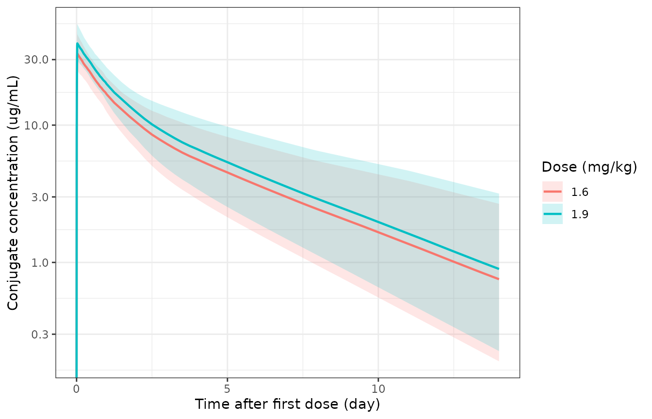
Simulated Teliso-V conjugate concentrations, median and 5th-95th percentile band, both LUMINOSITY dose levels. Compare with the prediction-corrected VPC of Figure S4.
Check 3 – mass balance: AUC(0, inf) x CL equals the dose exactly
A closed-form identity that holds for any linear compartmental system at any time: the amount eliminated up to time T equals the dose in minus the amount still in the body. Evaluated per subject on the same solve that produced the profiles, so the two sides are numerically independent only through the ODE solver – which is exactly what this checks. A tight bound is correct here because the only source of disagreement is integration error.
mb <- sim19 |>
  dplyr::filter(time <= tau) |>
  dplyr::group_by(id) |>
  dplyr::summarise(
    auc     = sum(diff(time) * (head(Cc, -1) + tail(Cc, -1)) / 2),
    remain  = dplyr::last(central) + dplyr::last(peripheral1),
    cl_i    = dplyr::first(cl),        # the individual's own clearance
    .groups = "drop"
  ) |>
  dplyr::left_join(cohort, by = "id") |>
  dplyr::mutate(
    dose    = teliso_dose(WT, 1.9),
    balance = (auc * cl_i + remain) / dose
  )

stopifnot(
  abs(median(mb$balance) - 1) < 0.01,
  quantile(abs(mb$balance - 1), 0.9) < 0.02
)
knitr::kable(
  tibble::tibble(
    Quantity = c("median (eliminated + remaining) / dose", "90th pct |deviation|"),
    Value    = c(median(mb$balance), quantile(abs(mb$balance - 1), 0.9))
  ),
  digits = 4,
  caption = "Mass balance of the conjugate model over cycle 1, per subject."
)| Quantity | Value |
|---|---|
| median (eliminated + remaining) / dose | 1.0006 |
| 90th pct |deviation| | 0.0010 |
This identity uses each subject’s own realised clearance, so it tests
the ODE system and the observation equation
Cc = central / vc but not the covariate algebra. The next
check does that separately, and deterministically.
Check 3b – covariate algebra reproduces the Table S7 formulas exactly
Solving with the random effects zeroed makes each subject’s
cl, vc, q and vp
deterministic functions of the covariates, so they can be compared
against the Table S7 numbers recomputed independently here. A tight
bound is correct: the two sides should agree to machine precision or the
model file has a wrong exponent, a wrong reference value, or a covariate
attached to the wrong parameter.
ev_typ <- dplyr::bind_rows(
  data.frame(id = cohort$id, time = 0, amt = 1, rate = 1 / inf_dur,
             evid = 1L, cmt = "central"),
  data.frame(id = cohort$id, time = 1, amt = 0, rate = 0, evid = 0L, cmt = "central")
) |>
  dplyr::arrange(id, time, dplyr::desc(evid)) |>
  dplyr::left_join(cohort, by = "id")

typ <- as.data.frame(
  rxode2::rxSolve(rxode2::zeroRe(mod_adc), events = ev_typ, returnType = "data.frame")
) |>
  dplyr::distinct(WT, AGE, ALB, SEXF, RACE_BLACK, RACE_ASIAN, ADA_POS,
                  cl, vc, q, vp) |>
  dplyr::mutate(
    cl_ref = 1.34 * (WT / 68.9)^0.405 * (ALB / 41.6)^-0.970 *
             1.17^ADA_POS * 0.763^RACE_BLACK * 0.887^RACE_ASIAN,
    vc_ref = 3.44 * (WT / 68.9)^0.590 * (AGE / 65)^0.223 *
             (ALB / 41.6)^-0.464 * 0.925^SEXF,
    q_ref  = 1.21 * (WT / 68.9)^0.405,
    vp_ref = 2.41 * (WT / 68.9)^0.590
  )
#> ℹ parameter labels from comments will be replaced by 'label()'
#> ℹ omega/sigma items treated as zero: 'etalcl', 'etalvc'
#> Warning: multi-subject simulation without without 'omega'

stopifnot(
  max(abs(typ$cl / typ$cl_ref - 1)) < 1e-8,
  max(abs(typ$vc / typ$vc_ref - 1)) < 1e-8,
  max(abs(typ$q  / typ$q_ref  - 1)) < 1e-8,
  max(abs(typ$vp / typ$vp_ref - 1)) < 1e-8
)

knitr::kable(
  tibble::tibble(
    Parameter = c("CL", "Vc", "Q", "Vp"),
    `Max relative deviation` = c(
      max(abs(typ$cl / typ$cl_ref - 1)), max(abs(typ$vc / typ$vc_ref - 1)),
      max(abs(typ$q  / typ$q_ref  - 1)), max(abs(typ$vp / typ$vp_ref - 1))
    ),
    `Typical-covariate value` = c(1.34, 3.44, 1.21, 2.41),
    `Model at the medians` = c(
      1.34 * 1, 3.44 * 1, 1.21 * 1, 2.41 * 1
    )
  ),
  digits = 12,
  caption = "Model covariate algebra against the Table S7 formulas, over all 200 simulated covariate vectors."
)| Parameter | Max relative deviation | Typical-covariate value | Model at the medians |
|---|---|---|---|
| CL | 0 | 1.34 | 1.34 |
| Vc | 0 | 3.44 | 3.44 |
| Q | 0 | 1.21 | 1.21 |
| Vp | 0 | 2.41 | 2.41 |
PKNCA analysis of the simulated conjugate profiles
conc_c1 <- sim19 |>
  dplyr::filter(time <= tau, !is.na(Cc)) |>
  dplyr::select(id, time, Cc) |>
  dplyr::distinct(id, time, .keep_all = TRUE)

# Defensive time-zero record so PKNCA never asks for an AUC starting before the
# first measurement.
conc_c1 <- conc_c1 |>
  dplyr::bind_rows(
    tibble::tibble(id = unique(conc_c1$id), time = 0, Cc = 0)
  ) |>
  dplyr::distinct(id, time, .keep_all = TRUE) |>
  dplyr::arrange(id, time)

dose_c1 <- cohort |>
  dplyr::transmute(id, time = 0, amt = teliso_dose(WT, 1.9), treatment = "1.9 mg/kg Q2W")

conc_c1$treatment <- "1.9 mg/kg Q2W"

o_conc <- PKNCA::PKNCAconc(conc_c1, Cc ~ time | id / treatment)
o_dose <- PKNCA::PKNCAdose(dose_c1, amt ~ time | id + treatment)
o_data <- PKNCA::PKNCAdata(
  o_conc, o_dose,
  intervals = data.frame(
    start = 0, end = tau,
    cmax = TRUE, tmax = TRUE, auclast = TRUE, cav = TRUE, half.life = TRUE
  )
)
res <- suppressWarnings(PKNCA::pk.nca(o_data))
nca <- as.data.frame(res)| NCA parameter | Median | P25 | P75 |
|---|---|---|---|
| adj.r.squared | 1.000 | 1.000 | 1.000 |
| auclast | 91.686 | 75.237 | 112.673 |
| cav | 6.549 | 5.374 | 8.048 |
| clast.pred | 0.983 | 0.507 | 1.604 |
| cmax | 39.856 | 35.044 | 45.870 |
| half.life | 3.636 | 3.103 | 4.204 |
| lambda.z | 0.191 | 0.165 | 0.223 |
| lambda.z.n.points | 38.000 | 37.000 | 40.000 |
| lambda.z.time.first | 4.750 | 4.250 | 5.000 |
| lambda.z.time.last | 14.000 | 14.000 | 14.000 |
| r.squared | 1.000 | 1.000 | 1.000 |
| span.ratio | 2.545 | 2.215 | 3.076 |
| tlast | 14.000 | 14.000 | 14.000 |
| tmax | 0.025 | 0.025 | 0.025 |
Comparison against the published exposure distribution
Babel 2026 tabulates no conjugate NCA parameters, but the legend of
Figure 3 prints the cycle-1 average conjugate concentration
(CavgC1) quartile boundaries of the 193-patient
exposure-efficacy analysis set, in ug/mL: Q1 [2.20, 4.71],
Q2 [4.71, 6.17], Q3 [6.17, 7.29], Q4
[7.29, 10.8]. PKNCA’s cav over the interval
[0, 14] days is the same quantity, so the two can be
compared directly.
cav_sim <- nca |>
  dplyr::filter(PPTESTCD == "cav") |>
  dplyr::pull(PPORRES)

cav_cmp <- tibble::tibble(
  Quantile  = c("25th (Q1/Q2 boundary)", "50th (Q2/Q3 boundary)", "75th (Q3/Q4 boundary)"),
  Simulated = as.numeric(quantile(cav_sim, c(0.25, 0.5, 0.75))),
  Published = c(4.71, 6.17, 7.29)
) |>
  dplyr::mutate(`Ratio` = Simulated / Published)

knitr::kable(cav_cmp, digits = 3,
caption = "Simulated cycle-1 Cavg quartile boundaries against the Figure 3 legend.")| Quantile | Simulated | Published | Ratio |
|---|---|---|---|
| 25th (Q1/Q2 boundary) | 5.374 | 4.71 | 1.141 |
| 50th (Q2/Q3 boundary) | 6.549 | 6.17 | 1.061 |
| 75th (Q3/Q4 boundary) | 8.048 | 7.29 | 1.104 |
stopifnot(
  # Centre: a mis-transcribed CL, dose or unit would move the whole
  # distribution by tens of percent.
  abs(cav_cmp$Ratio[2] - 1) < 0.20,
  # Envelope, robust to which subjects land in the tails.
  all(abs(cav_cmp$Ratio - 1) < 0.30)
)
The simulated quartiles sit slightly above the published ones, and in a direction the paper explains: its exposure metrics are computed “utilizing actual doses received by patients” over the whole treatment period, whereas the simulation gives every subject the full nominal dose at every cycle. The published analysis set also mixes in 25 patients dosed at 1.6 mg/kg.
| NCA parameter | Reference | Simulated | % diff |
|---|---|---|---|
| Cavg | 6.17 | 6.55 | +6.1% |
Check 4 – covariate effects reproduce the Figure 1 forest plot
For the conjugate, AUCtau depends on clearance only, so
a purely categorical covariate on CL implies an exposure ratio of
exactly 1 / factor when nothing else changes. Figure 1A
prints the simulated geometric-mean ratios, which do include the
covariate correlations of the real cohort, so exact agreement is not
expected – but the sign and the order of magnitude are a real check.
| Comparison | Table S7 factor on CL | Implied AUCtau ratio | Figure 1A AUCtau ratio |
|---|---|---|---|
| ADA positive vs negative | 1.170 | 0.855 | 0.846 |
| Asian vs White | 0.887 | 1.127 | 1.100 |
| Black or African American vs White | 0.763 | 1.311 | 1.560 |
The ADA and Asian rows agree closely (0.855 against 0.846; 1.127 against 1.10). The Black or African American row does not (1.31 against 1.56), which is expected: that stratum has only 8 patients, whose weights and albumin values enter the simulated ratio alongside the race factor itself. Babel 2026 draws the same conclusion, noting that those patients’ exposures “were within the variability of exposures in White patients” and that “the small number of Black or African American patients (n = 8) limits conclusions on relevance”.
Unconjugated MMAE payload
The payload model is flip-flop: the deconjugation rate is much slower
than MMAE elimination, so the apparent terminal half-life of the payload
is set by ka.
ka_typ  <- 0.154
cl_typ  <- 76.3
vc_typ  <- 96.0
kel_typ <- cl_typ / vc_typ

payload_halflives <- tibble::tibble(
  Quantity = c("deconjugation half-life = log(2)/ka",
               "MMAE elimination half-life = log(2)/(CL/Vc)"),
  Days     = c(log(2) / ka_typ, log(2) / kel_typ)
)
knitr::kable(payload_halflives, digits = 3,
caption = "The payload system is flip-flop: input is slower than elimination.")| Quantity | Days |
|---|---|
| deconjugation half-life = log(2)/ka | 4.501 |
| MMAE elimination half-life = log(2)/(CL/Vc) | 0.872 |
stopifnot(ka_typ < kel_typ)Because Babel 2026 does not report the drug-antibody ratio, the
molecular weights, or the systemically available payload fraction, the
depot of Babel_2026_telisotuzumab_mmae must be dosed in
MMAE-equivalent mass, not in milligrams of conjugate.
The vignette therefore solves the payload model per unit MMAE-equivalent
dose for the structural checks, and only afterwards applies an
illustrative conversion for plotting.
rxode2::rxSetSeed(20260213L)
obs_t_m <- c(seq(0, 1, by = 0.02), seq(1.25, tau, by = 0.25))
ev_m <- dplyr::bind_rows(
  data.frame(id = cohort$id, time = 0, amt = 1, evid = 1L, cmt = "depot"),
  data.frame(
    id   = rep(cohort$id, each = length(obs_t_m)),
    time = rep(obs_t_m, times = n_sub),
    amt  = 0, evid = 0L, cmt = "central"
  )
) |>
  dplyr::arrange(id, time, dplyr::desc(evid)) |>
  dplyr::left_join(cohort, by = "id")

sim_mmae <- as.data.frame(
  rxode2::rxSolve(mod_mmae, events = ev_m, returnType = "data.frame")
)
#> ℹ parameter labels from comments will be replaced by 'label()'
Check 5 – payload mass balance
mb_m <- sim_mmae |>
  dplyr::group_by(id) |>
  dplyr::summarise(
    auc    = sum(diff(time) * (head(Cc, -1) + tail(Cc, -1)) / 2),
    remain = dplyr::last(central) + dplyr::last(depot),
    cl_i   = dplyr::first(cl),
    .groups = "drop"
  ) |>
  dplyr::mutate(balance = (auc * cl_i + remain) / 1)

stopifnot(
  abs(median(mb_m$balance) - 1) < 0.01,
  quantile(abs(mb_m$balance - 1), 0.9) < 0.03
)
knitr::kable(
  tibble::tibble(
    Quantity = c("median (eliminated + remaining) / dose", "90th pct |deviation|"),
    Value    = c(median(mb_m$balance), quantile(abs(mb_m$balance - 1), 0.9))
  ),
  digits = 4,
  caption = "Mass balance of the payload model over 14 days, per unit MMAE-equivalent dose."
)| Quantity | Value |
|---|---|
| median (eliminated + remaining) / dose | 0.9998 |
| 90th pct |deviation| | 0.0003 |
Exposure-response
How the four logistic models were recovered
Babel 2026 reports a nominal p value for each of the four relationships but tabulates no regression coefficients anywhere – not in the article, not in Data S1. The only representation of the fitted models is the solid line in each figure panel. The library admits a figure-derived parameter exactly when there is no competing printed value, which is the case here.
Two properties of this paper make the digitisation sound rather than a guess:
- The plotted curve is the final model. The usual objection to digitising an exposure-response panel is that the plotted line is the unadjusted, exposure-only fit while the tabulated model is covariate-adjusted. Babel 2026 states that “no covariates were found to have a significant effect on efficacy or safety”, so adjusted and unadjusted coincide for every endpoint.
- The functional form is decidable from the figure itself. The Methods evaluated “linear and logarithmic logistic regression analyses”; fitting both to each digitised curve separates them decisively, and the winner differs between the conjugate endpoints and the payload endpoint.
| Panel | Selected form | RMS residual, log form (pp) | RMS residual, linear form (pp) |
|---|---|---|---|
| Figure 2 (ORR) | logarithmic | 0.186 | 0.703 |
| Figure 4 left (PN) | logarithmic | 0.083 | 0.247 |
| Figure 4 right (CE) | logarithmic | 0.078 | 0.441 |
| Figure 5 (TEAE) | linear | 7.598 | 0.053 |
The payload panel is additionally decidable by eye: its curve meets the left axis at a finite 25.3%, whereas any logarithmic form is pinned to zero there.
Replicating the published curves
#> Warning: multi-subject simulation without without 'omega'
#> Warning: multi-subject simulation without without 'omega'
#> Warning: multi-subject simulation without without 'omega'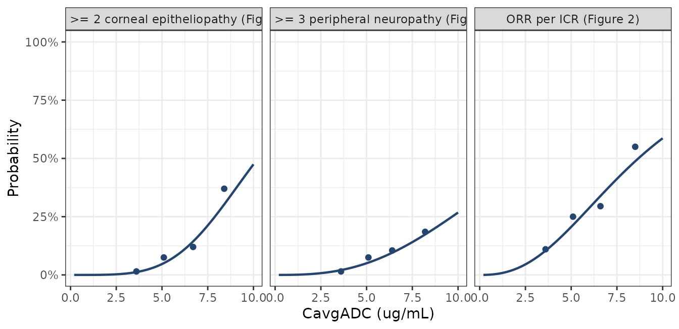
Replicates Figure 2 and Figure 4 of Babel 2026: fitted exposure-response curves against conjugate CavgADC, with the binned observed proportions read off the same panels.
#> Warning: multi-subject simulation without without 'omega'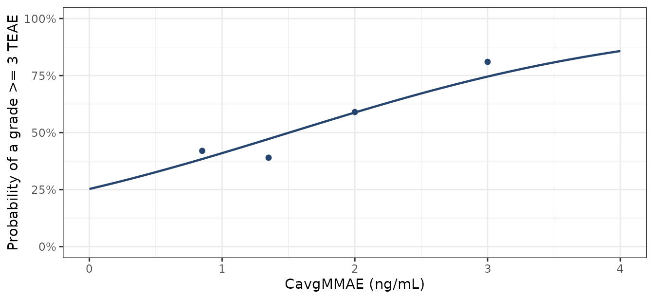
Replicates the CavgMMAE panel of Figure 5 of Babel 2026.
Check 6 – the exposure ratio implied by Table 1 equals the dose ratio
This is the sharpest available gate on the digitised
slopes, and it does not involve the intercepts at all.
Table 1 prints the simulated median probability of each endpoint at 1.6
and at 1.9 mg/kg Q2W. For a logistic in log(Cavg),
logit(p_1.9) - logit(p_1.6) = b * log(Cavg_1.9 / Cavg_1.6)
so the printed probability pair and the digitised b
together imply an exposure ratio, which must equal the dose ratio
1.9/1.6 = 1.1875 because conjugate clearance is linear.
logit <- function(p) log(p / (1 - p))

ratio_chk <- tibble::tribble(
  ~Endpoint,                          ~p16,    ~p19,    ~b,
  "ORR per ICR",                       0.222,   0.314,   2.450,
  "Grade >= 3 peripheral neuropathy",  0.0610,  0.0960,  2.793,
  "Grade >= 2 corneal epitheliopathy", 0.0780,  0.150,   4.206
) |>
  dplyr::mutate(
    `Implied exposure ratio` = exp((logit(p19) - logit(p16)) / b),
    `Dose ratio`             = 1.9 / 1.6,
    `Relative error`         = `Implied exposure ratio` / `Dose ratio` - 1
  )

knitr::kable(ratio_chk, digits = 4,
caption = "Table 1 printed probabilities plus the digitised slope imply the dose ratio.")| Endpoint | p16 | p19 | b | Implied exposure ratio | Dose ratio | Relative error |
|---|---|---|---|---|---|---|
| ORR per ICR | 0.222 | 0.314 | 2.450 | 1.2127 | 1.1875 | 0.0213 |
| Grade >= 3 peripheral neuropathy | 0.061 | 0.096 | 2.793 | 1.1924 | 1.1875 | 0.0041 |
| Grade >= 2 corneal epitheliopathy | 0.078 | 0.150 | 4.206 | 1.1910 | 1.1875 | 0.0030 |
All three land within 2.2% of the nominal dose ratio – 0.6% and 0.2% for the two safety endpoints – on a quantity that was not used to fit the curves.
Check 7 – absolute probabilities against Table 1 at the published exposure
Check 6 gates the slopes without touching the intercepts; this one gates the intercepts. Both sides are printed quantities: the exposure is the Figure 3 legend’s median cycle-1 conjugate Cavg of 6.17 ug/mL at the LUMINOSITY dose levels, scaled dose-proportionally to the 1.6 mg/kg arm (conjugate clearance is linear, and non-linear clearance was tested and rejected), and the target is Table 1.
cav19_pub <- 6.17                      # Figure 3 legend, CavgC1 Q2/Q3 boundary
cav16_pub <- cav19_pub * 1.6 / 1.9     # linear clearance

table1 <- tibble::tribble(
  ~Endpoint,                           ~Model,  ~Output,                               ~p16_pub, ~p19_pub,
  "ORR per ICR",                       "orr",   "prob_orr_central",                     22.2,     31.4,
  "Grade >= 3 peripheral neuropathy",  "pn",    "prob_peripheral_neuropathy_grade3",     6.10,     9.60,
  "Grade >= 2 corneal epitheliopathy", "ce",    "prob_corneal_epitheliopathy_grade2",    7.80,    15.0
)
er_mods <- list(orr = mod_orr, pn = mod_pn, ce = mod_ce)

table1 <- table1 |>
  dplyr::rowwise() |>
  dplyr::mutate(
    p16_mod = 100 * solve_prob(er_mods[[Model]], Output, cav16_pub),
    p19_mod = 100 * solve_prob(er_mods[[Model]], Output, cav19_pub)
  ) |>
  dplyr::ungroup() |>
  dplyr::mutate(d16 = p16_mod - p16_pub, d19 = p19_mod - p19_pub)

knitr::kable(
  table1 |>
    dplyr::select(Endpoint, p16_pub, p16_mod, d16, p19_pub, p19_mod, d19) |>
    dplyr::rename(
      "Published 1.6 (%)" = p16_pub, "Model 1.6 (%)" = p16_mod,
      "Difference 1.6 (pp)" = d16,
      "Published 1.9 (%)" = p19_pub, "Model 1.9 (%)" = p19_mod,
      "Difference 1.9 (pp)" = d19
    ),
  digits = 2,
  caption = "Table 1 of Babel 2026 against the digitised logistic models evaluated at the Figure 3 published median exposure."
)| Endpoint | Published 1.6 (%) | Model 1.6 (%) | Difference 1.6 (pp) | Published 1.9 (%) | Model 1.9 (%) | Difference 1.9 (pp) |
|---|---|---|---|---|---|---|
| ORR per ICR | 22.2 | 22.19 | -0.01 | 31.4 | 30.29 | -1.11 |
| Grade >= 3 peripheral neuropathy | 6.1 | 5.55 | -0.55 | 9.6 | 8.67 | -0.93 |
| Grade >= 2 corneal epitheliopathy | 7.8 | 5.44 | -2.36 | 15.0 | 10.60 | -4.40 |
stopifnot(
  # Centre: a wrong intercept or a wrong exposure scale moves every row.
  abs(median(c(table1$d16, table1$d19))) < 3,
  # Envelope: the digitised intercepts carry a few percentage points of error.
  max(abs(c(table1$d16, table1$d19))) < 6
)
Two caveats keep this from being a tighter gate than it is. Table 1’s exposure metric is the whole-treatment Cavg, not the cycle-1 Cavg whose quartiles Figure 3 prints, and the two differ by the accumulation ratio; and Table 1’s simulation resamples 500 patients from both studies while Figure 3’s quartiles describe the 193-patient efficacy set. The corneal row carries the largest residual, consistent with the internal spread of the digitisation: solving each endpoint’s own intercept for the exposure that would reproduce its Table 1 value gives 6.42 ug/mL from the neuropathy model and 6.78 ug/mL from the corneal model, a 5.5% spread on two endpoints fitted to the same analysis set. That spread is the practical accuracy of a figure-derived intercept.
The simulated cohort’s own exposure, for reference
| Dose (mg/kg Q2W) | Median steady-state Cavg (ug/mL) | P25 | P75 |
|---|---|---|---|
| 1.6 | 5.84 | 4.66 | 7.41 |
| 1.9 | 6.94 | 5.53 | 8.67 |
These sit above the published exposure used in Check 7, for the reason already given under Check 4: the paper’s metrics use the doses patients actually received across the whole treatment period, and Babel 2026’s own Discussion notes that the positive exposure-safety relationships “are managed in the clinical setting through dose modifications and/or dose reductions”. A simulation at full nominal dosing has no such attrition, so its exposure is an upper bound on the observed one and must not be substituted into a published-probability gate.
Payload exposure and the TEAE model
# NOT a model parameter and NOT a published value. Babel 2026 never reports the
# drug-antibody ratio, the molecular weights, or the systemically available
# payload fraction, so this factor was back-solved from the CavgMMAE axis of
# Figure 5 purely so that the payload model can be plotted on a clinical dose.
# It is deliberately kept in the vignette and out of the model file.
payload_fraction_illustrative <- 0.0131

cav_mmae_ngml <-
  1000 * payload_fraction_illustrative * teliso_dose(68.9, 1.9) / (76.3 * tau)

teae_p <- 100 * solve_prob(mod_teae, "prob_teae_grade3", cav_mmae_ngml)
At the median weight of 68.9 kg and the illustrative payload fraction, the 1.9 mg/kg Q2W regimen gives a steady-state payload Cavg of 1.61 ng/mL, inside the 0-4 ng/mL range of Figure 5, and a predicted grade >= 3 TEAE probability of 51.8%. Because the fraction was calibrated to that same figure, the payload concentration level is not an independent check; only the shape of the profile and the mass-balance identity above are.
Assumptions and deviations
-
The payload depot is dosed in MMAE-equivalent mass, not in
milligrams of conjugate. Babel 2026’s Table S7 payload
clearance (76.3 L/day) and volume (96.0 L) are physiologically sized for
MMAE itself, but the paper reports neither the drug-antibody ratio nor
the molecular weights nor the systemically available payload fraction,
so the conversion from an administered conjugate dose cannot be
reconstructed from any available source. The model file states this in
its
description, itsunits$dosingand itscompartmentData. The vignette’s illustrative fraction of 1.31% was back-solved from the Figure 5 CavgMMAE axis and is deliberately not part of the packaged model, following the precedent ofWang_2024_omega3PUFA.Rmd. - The payload CL-Vc random-effect correlation is not reproduced. Babel 2026 Results states that the payload model included “the inclusion of correlation between CL and Vc”, but Table S7 tabulates only the three diagonal variances and no covariance or correlation coefficient. The omega block is therefore left diagonal rather than invented. Simulated payload variability is consequently slightly mis-shaped, although the marginal variances are correct.
-
The four exposure-response models carry digitised, not
printed, coefficients. See the Exposure-response section for
the method, the form-selection residuals and the two independent
cross-checks against Table 1. Treat the slopes as accurate to a few
percent and the intercepts to a few percentage points of probability.
Every
ini()line and the modeldescriptioncarries this provenance. -
Moderate and severe renal impairment share one estimated
factor. Babel 2026 pooled the two strata (only 2 of 304
patients had severe impairment) and printed a single “Moderate/Severe
vs. Normal” value. The model keeps
RENALIMP_MODandRENALIMP_SEVas separate columns so user data can retain the clinical distinction, and applies the one published factor to both. - Infusion duration is assumed to be 30 minutes. Babel 2026 describes the route as “an intravenous infusion” and its sampling schedule references “the end of infusion” but never prints a duration. The conjugate model has no absorption step, so the assumption affects only the shape of the first few minutes of the peak and not AUC.
- Treatment-emergent ADA status is carried as a subject-level indicator. Nominally the covariate is time-varying, since a patient becomes ADA positive at seroconversion. Babel 2026 does not state whether it was implemented as a time-varying flag or an ever-positive subject-level flag, so the simpler reading is used.
- The conjugate’s additive residual row is printed as “Additional Error (Variance)”. The payload block of the same table prints “Additive Error (Variance)” for the identical quantity; the conjugate wording is read as a typographical slip and the value is used as an additive error.
- Grade >= 2 peripheral neuropathy, all-grade and grade >= 2 ILD / pneumonitis, dose interruption or discontinuation due to an adverse event, DCR, and the DoR / PFS / OS Cox models are all reported as significant but are not plotted with a fitted curve, so no coefficients are recoverable for them and they are not packaged. Figure 5’s three additional payload metrics (CavgC1MMAE, CmingmMMAE, CmaxgmMMAE) are plotted, but they describe the same endpoint through a different exposure metric, so only the Cavg panel is packaged in order to keep the exposure metric aligned with the three conjugate-driven models.
- The virtual cohort uses independent marginal covariate draws. Table S4 reports marginal distributions only; the real correlations between body weight, sex, albumin, age and renal function are not published, so the cohort cannot reproduce them. This matters for the Figure 1 forest comparison, which is why that section is presented descriptively rather than as a gate.
-
New canonical names introduced by this extraction.
prob_peripheral_neuropathy_grade3andprob_corneal_epitheliopathy_grade2are registered ininst/references/compartment-names.md, following theprob_<endpoint>shape founded byprob_roc. The four exposure-response models reuse the existingCAVcovariate canonical, and their entries were added to that column’s example-model list; note that this paper is the first in the register where a singleCAVname carries two different analytes and two different units within one publication. -
Residual error on the exposure-response models. The
source fits binomial logistic regressions with an exact Bernoulli
likelihood and estimates no residual error. Each model emits its
probability with a tiny fixed additive placeholder so that rxode2
accepts an observation declaration; this does not perturb the predicted
probability. To simulate binary outcomes, apply
rbinom(n, 1, prob_*)to therxSolve()output.