Tobramycin in rats with acute or chronic Pseudomonas lung infection (Dias 2022)
Source:vignettes/articles/Dias_2022_tobramycin_rat.Rmd
Dias_2022_tobramycin_rat.Rmd
mod <- rxode2::rxode2(readModelDb("Dias_2022_tobramycin_rat"))
#> ℹ parameter labels from comments will be replaced by 'label()'
Model and source
- Citation: Dias BB, Carreno F, Helfer VE, Garzella PMB, de Lima DMF, Barreto F, de Araujo BV, Dalla Costa T. Probability of Target Attainment of Tobramycin Treatment in Acute and Chronic Pseudomonas aeruginosa Lung Infection Based on Preclinical Population Pharmacokinetic Modeling. Pharmaceutics. 2022;14(6):1237. doi:10.3390/pharmaceutics14061237. PMCID: PMC9228144. Parameter estimates: Table 1. Structural ODEs: Equations 1-3. Lung, ELF and unbound-fraction observation equations: Results text after Equation 3. Group sizes: Supplementary Table S2. Human-to-rat dose scaling: Supplementary Equations S1-S2 and Table S1.
- Description: Preclinical (rat, Wistar male). Three-compartment population PK model for intravenous tobramycin in healthy rats and in rats with acute or chronic biofilm-forming Pseudomonas aeruginosa lung infection, fit jointly to total plasma concentrations and to unbound lung and epithelial-lining-fluid (ELF) concentrations measured by microdialysis. The ODE states carry UNBOUND drug amounts: central (plasma), peripheral1 and a third lung compartment (the lung interstitial space sampled by the lung microdialysis probe). Unbound ELF concentration is the unbound lung concentration times a distribution factor (Dfactor), and total plasma is unbound plasma divided by the unbound fraction 0.89. Chronic infection (alginate beads carrying P. aeruginosa ATCC 27853) has its own clearance and central volume; every intratracheally inoculated group (acute PA14 infection, chronic infection and sterile blank alginate beads) shares a larger lung volume than healthy rats.
- Article: https://doi.org/10.3390/pharmaceutics14061237 (PMC9228144, open access)
- Supplementary Materials (Tables S1-S2, Equations S1-S2): https://www.mdpi.com/article/10.3390/pharmaceutics14061237/s1
Dias et al. gave male Wistar rats a single 10 mg/kg intravenous bolus
of tobramycin and measured total plasma concentrations together with
unbound lung-interstitial and unbound epithelial-lining-fluid (ELF)
concentrations by microdialysis. The final model (Figure 1 of the paper)
has three compartments: central (plasma), a peripheral compartment, and
a lung compartment whose unbound concentration is what the lung
microdialysis probe samples. ELF is not a compartment: unbound ELF
concentration is the unbound lung concentration times a distribution
factor, Dfactor.
Population
| Field | Value |
|---|---|
| Species | rat (Wistar, male) |
| Animals | 71 |
| Studies | 1 |
| Weight | 200-250 g |
| Female | 0% |
| Groups | Four groups: healthy; acute P. aeruginosa PA14 lung infection (7 days after intratracheal inoculation); chronic P. aeruginosa ATCC 27853 lung infection established with bacteria-laden alginate beads (14 days after inoculation); and a blank-bead control inoculated with sterile alginate beads. |
| Dose | Single 10 mg/kg intravenous bolus through the femoral vein. |
| Region | Brazil (Federal University of Rio Grande do Sul, Porto Alegre) |
The 1231 observations from 71 rats come from four experimental groups (Section 2.3; animal and observation counts per group and matrix in Supplementary Table S2):
- healthy rats;
- acute infection: intratracheal planktonic P. aeruginosa PA14, PK studied 7 days later;
- chronic infection: intratracheal alginate beads carrying P. aeruginosa ATCC 27853 (a model of the mucoid chronic infection of cystic-fibrosis airways), PK studied 14 days later;
- blank bead: intratracheal sterile alginate beads, the control for the alginate matrix itself.
The groups are encoded by three mutually exclusive indicators,
DIS_PSEUDOMONAS_LUNG_ACUTE,
DIS_PSEUDOMONAS_LUNG_CHRONIC and
ALGINATE_BEAD_BLANK; a healthy rat has all three at 0.
Source trace
Every value below is the final estimate printed in Table 1 of the paper.
| Model element | Value in file | Source location |
|---|---|---|
d/dt(central) |
-(Q1/V1 + Q2/V1 + CL/V1) A1 + Q1/V2 A2 + Q2/V3 A3 | Equation 1 |
d/dt(peripheral1) |
-Q1/V2 A2 + Q1/V1 A1 | Equation 2 |
d/dt(lung) |
-Q2/V3 A3 + Q2/V1 A1 | Equation 3 |
Clung (unbound lung) |
A3 / V3 | Results, after Equation 3 |
Celf (unbound ELF) |
(A3 / V3) x Dfactor | Results, after Equation 3 |
Cc (total plasma) |
(A1 / V1) / 0.89 | Results, after Equation 3; Methods 2.5 (11% protein binding) |
lcl_nonchronic |
log(0.047) L/h | Table 1, CL |
lcl_chronic |
log(0.085) L/h | Table 1, CLchronic |
lvc_nonchronic |
log(0.055) L | Table 1, V1 |
lvc_chronic |
log(0.323) L | Table 1, V1chronic |
lq |
log(0.030) L/h | Table 1, Q1 |
lvp |
log(0.154) L | Table 1, V2 |
lq_lung |
log(0.370) L/h | Table 1, Q2 |
lv_lung_healthy |
log(0.083) L | Table 1, V3 |
lv_lung_inoc |
log(0.130) L | Table 1, V3infected; Results (“Acute, chronic, and blank-bead were included as covariates in V3”) |
lr_elf_lung |
log(0.36) | Table 1, Dfactor |
fu |
0.89 (fixed) | Results, after Equation 3 |
etalcl |
0.5339 = log(0.84^2 + 1) | Table 1, omega CL 84 %CV |
etalvc |
0.3075 = log(0.60^2 + 1) | Table 1, omega V1 60 %CV |
etalv_lung |
1.0280 = log(1.34^2 + 1) | Table 1, omega V3 134 %CV |
etalr_elf_lung |
0.1697 = log(0.43^2 + 1) | Table 1, omega Dfactor 43 %CV |
expSd |
0.152 | Table 1, plasma log-additive error |
expSd_Clung, expSd_Celf
|
0.313 each | Table 1, microdialysis log-additive error (one estimate shared by lung and ELF) |
Dimensional check: with doses in mg, volumes in L and clearances in L/h, every term of Equations 1-3 is in mg/h and every concentration is in mg/L.
Single 10 mg/kg bolus: the four groups
The experiments gave 10 mg/kg as an intravenous bolus. A 0.25 kg rat (the top of the 200-250 g study range) receives 2.5 mg. The cohort below has 100 virtual rats per group.
rat_wt <- 0.25 # kg
n_per_group <- 100L

bolus_events <- function(grp, id_offset) {
  ev <- rxode2::et(amt = 10 * rat_wt, cmt = "central") |>
    rxode2::et(c(seq(0, 2, by = 0.05), seq(2.25, 12, by = 0.25), seq(13, 72, by = 1)),
               cmt = "central") |>
    as.data.frame()
  # Three ~ endpoints: observation rows need a dvid; dvid = 1 still returns
  # every model variable (Cc, Cu, Clung, Celf) as a column.
  ev$dvid <- ifelse(ev$evid == 0, 1L, NA_integer_)
  cohort <- tidyr::crossing(id = seq_len(n_per_group) + id_offset, ev)
  dplyr::bind_cols(cohort, dplyr::select(grp, -group)[rep(1, nrow(cohort)), ]) |>
    mutate(group = grp$group)
}

bolus_ev <- dplyr::bind_rows(lapply(seq_len(nrow(groups)), function(i) {
  bolus_events(groups[i, ], (i - 1L) * n_per_group)
})) |>
  arrange(id, time, desc(evid))

rxode2::rxSetSeed(2022)
bolus_sim <- rxode2::rxSolve(mod, bolus_ev, keep = "group", useLinCmt = FALSE) |>
  as.data.frame()
# Typical values: omega = NA, sigma = NA (one rat per group).
bolus_typ <- rxode2::rxSolve(mod,
                             bolus_ev |> filter(id %in% ((seq_len(nrow(groups)) - 1L) * n_per_group + 1L)),
                             keep = "group", useLinCmt = FALSE, omega = NA, sigma = NA) |>
  as.data.frame()

long_endpoints <- function(d) {
  d |>
    select(id, time, group, `Total plasma` = Cc, `Unbound lung` = Clung,
           `Unbound ELF` = Celf) |>
    pivot_longer(c(`Total plasma`, `Unbound lung`, `Unbound ELF`),
                 names_to = "matrix", values_to = "conc") |>
    mutate(matrix = factor(matrix, levels = c("Total plasma", "Unbound lung", "Unbound ELF")))
}
long_endpoints(bolus_typ) |>
  filter(dplyr::between(time, 0.05, 12)) |>
  ggplot(aes(time, conc, colour = group)) +
  geom_line(linewidth = 0.8) +
  facet_wrap(~matrix) +
  scale_y_log10() +
  labs(x = "Time after dose (h)", y = "Tobramycin (mg/L)", colour = "Group") +
  theme_bw() +
  theme(legend.position = "bottom")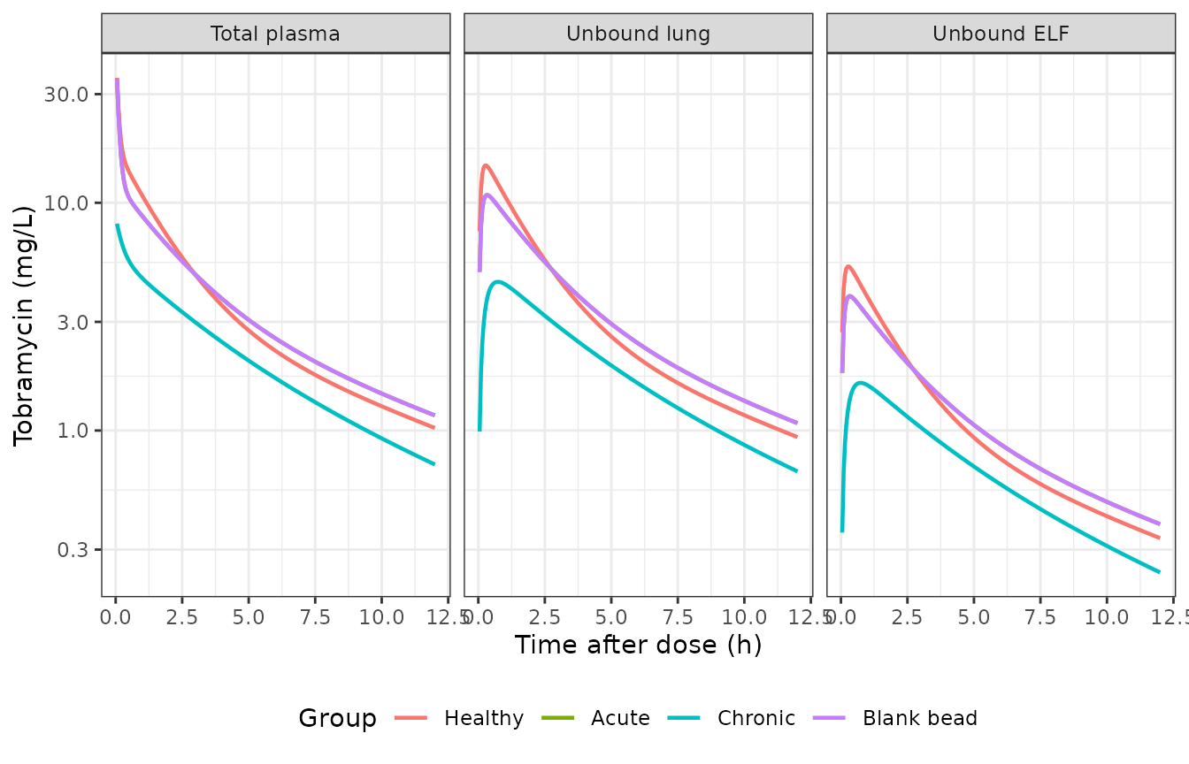
Typical-value profiles after a 10 mg/kg intravenous bolus in each group (compare with the observed profiles of Supplementary Figure S3).
The figure shows what Table 1 implies. Chronic infection raises clearance and the central volume, so its total plasma curve starts lower and falls more slowly. Every inoculated group (acute, chronic and blank bead) has the larger lung volume V3infected. Its unbound lung concentrations therefore rise more slowly and peak lower than in healthy rats. ELF tracks lung at a fixed 36%.
long_endpoints(bolus_sim) |>
  filter(dplyr::between(time, 0.05, 12)) |>
  group_by(group, matrix, time) |>
  summarise(p10 = quantile(conc, 0.1), p50 = median(conc), p90 = quantile(conc, 0.9),
            .groups = "drop") |>
  ggplot(aes(time, p50)) +
  geom_ribbon(aes(ymin = p10, ymax = p90), fill = "#1F6F7A", alpha = 0.25) +
  geom_line(colour = "#1F6F7A") +
  facet_grid(matrix ~ group, scales = "free_y") +
  scale_y_log10() +
  labs(x = "Time after dose (h)", y = "Tobramycin (mg/L)") +
  theme_bw()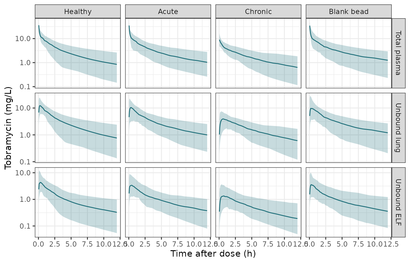
Simulated 10th, 50th and 90th percentiles (individual predictions, 100 rats per group) after a 10 mg/kg bolus, the percentiles used in the stratified pcVPC of Figure 2.
PKNCA
The paper reports no NCA, so PKNCA is used here as an internal
consistency check. For a linear model with elimination only from the
central compartment, the total-plasma AUC from zero to infinity must
equal dose / (CL x fu) for every simulated rat. The
comparison uses each rat’s own drawn clearance, so the only difference
is numerical (trapezoidal AUC plus the log-linear extrapolation past 72
h).
sim_nca <- bolus_sim |>
  filter(!is.na(Cc)) |>
  select(id, time, Cc, group)

conc_obj <- PKNCA::PKNCAconc(sim_nca, Cc ~ time | group + id)
dose_df <- bolus_ev |>
  filter(evid == 1) |>
  select(id, time, amt, group)
dose_obj <- PKNCA::PKNCAdose(dose_df, amt ~ time | group + id, route = "intravascular")

intervals <- data.frame(start = 0, end = Inf, cmax = TRUE, aucinf.obs = TRUE,
                        half.life = TRUE)
nca_res <- PKNCA::pk.nca(PKNCA::PKNCAdata(conc_obj, dose_obj, intervals = intervals))

nca_wide <- as.data.frame(nca_res$result) |>
  select(group, id, PPTESTCD, PPORRES) |>
  pivot_wider(names_from = PPTESTCD, values_from = PPORRES)

nca_wide |>
  group_by(group) |>
  summarise(cmax = median(cmax), aucinf.obs = median(aucinf.obs),
            half.life = median(half.life), .groups = "drop") |>
  mutate(across(c(cmax, aucinf.obs, half.life), \(x) signif(x, 3))) |>
  rename(Group = group, `Cmax (mg/L)` = cmax, `AUC0-inf (mg*h/L)` = aucinf.obs,
         `Terminal t1/2 (h)` = half.life) |>
knitr::kable(caption = "Median simulated total-plasma NCA after a 10 mg/kg bolus (0.25 kg rat).")| Group | Cmax (mg/L) | AUC0-inf (mg*h/L) | Terminal t1/2 (h) |
|---|---|---|---|
| Healthy | 51.40 | 51.7 | 6.50 |
| Acute | 52.90 | 55.3 | 7.57 |
| Chronic | 9.77 | 29.9 | 6.85 |
| Blank bead | 50.90 | 64.7 | 7.94 |
auc_check <- nca_wide |>
  left_join(bolus_sim |> distinct(id, cl), by = "id") |>
  mutate(auc_expected = 10 * rat_wt / (cl * 0.89),
         pct_diff = 100 * (aucinf.obs - auc_expected) / auc_expected)
stopifnot(
  nrow(auc_check) == nrow(groups) * n_per_group,
  !anyNA(auc_check$pct_diff),
  abs(median(auc_check$pct_diff)) < 2,
  quantile(abs(auc_check$pct_diff), 0.9) < 5
)
summary(auc_check$pct_diff)
#>     Min.  1st Qu.   Median     Mean  3rd Qu.     Max.
#> -0.61589  0.01112  0.03721  0.08945  0.10028  1.52499
Probability of target attainment (Figure 3)
The paper’s application was a probability-of-target-attainment (PTA) analysis. Human regimens were scaled to rats by body-surface allometry (Supplementary Equations S1-S2, Table S1): 1, 3, 10 and 11 mg/kg in humans become 3.8, 11.3, 37.2 and 41.4 mg/kg in rats. Each was given as a 30-min intravenous infusion, and the target was an unbound peak over MIC (fCmax/MIC) above 10. The text reports PTA at the most prevalent P. aeruginosa MIC of 0.5 mg/L, which means an unbound peak above 5 mg/L. The acute regimens were simulated with the acute-infection parameters and the chronic regimens with the chronic-infection parameters. The Discussion adds that 4.5 mg/kg q24h in humans (16.9 mg/kg in rats) is needed to reach 90% PTA in lung for acute infection.
The peak is taken over the third day of dosing, after any accumulation. There are 200 virtual rats per regimen.
n_pta <- 200L
regimens <- tibble::tribble(
  ~regimen,                    ~infection, ~human_mgkg, ~rat_mgkg, ~tau,
  "Acute, 1 mg/kg q8h",        "Acute",    1,           3.8,       8,
  "Acute, 3 mg/kg q24h",       "Acute",    3,           11.3,      24,
  "Acute, 4.5 mg/kg q24h",     "Acute",    4.5,         16.9,      24,
  "Chronic, 3 mg/kg q24h",     "Chronic",  3,           11.3,      24,
  "Chronic, 11 mg/kg q24h",    "Chronic",  11,          41.4,      24
)

pta_events <- function(i) {
  r <- regimens[i, ]
  grp <- groups |> filter(group == r$infection)
  ev <- rxode2::et(amt = r$rat_mgkg * rat_wt, dur = 0.5, ii = r$tau,
                   addl = 72 / r$tau - 1, cmt = "central") |>
    rxode2::et(seq(48, 72, by = 0.05), cmt = "central") |>
    as.data.frame()
  ev$dvid <- ifelse(ev$evid == 0, 1L, NA_integer_)
  cohort <- tidyr::crossing(id = seq_len(n_pta) + (i - 1L) * n_pta, ev)
  dplyr::bind_cols(cohort, dplyr::select(grp, -group)[rep(1, nrow(cohort)), ]) |>
    mutate(regimen = r$regimen)
}
pta_ev <- dplyr::bind_rows(lapply(seq_len(nrow(regimens)), pta_events)) |>
  arrange(id, time, desc(evid))

rxode2::rxSetSeed(2023)
pta_sim <- rxode2::rxSolve(mod, pta_ev, keep = "regimen", useLinCmt = FALSE) |>
  as.data.frame()

peaks <- pta_sim |>
  group_by(regimen, id) |>
  summarise(`Unbound plasma` = max(Cu), `Unbound lung` = max(Clung),
            `Unbound ELF` = max(Celf), .groups = "drop") |>
  pivot_longer(-c(regimen, id), names_to = "matrix", values_to = "fcmax")
published_pta <- tibble::tribble(
  ~regimen,                 ~matrix,          ~paper,
  "Acute, 1 mg/kg q8h",     "Unbound plasma", 90,
  "Acute, 1 mg/kg q8h",     "Unbound lung",   62.8,
  "Acute, 1 mg/kg q8h",     "Unbound ELF",    3.6,
  "Acute, 3 mg/kg q24h",    "Unbound plasma", 100,
  "Acute, 3 mg/kg q24h",    "Unbound lung",   85.6,
  "Acute, 3 mg/kg q24h",    "Unbound ELF",    15.8,
  "Chronic, 3 mg/kg q24h",  "Unbound plasma", 87.0,
  "Chronic, 3 mg/kg q24h",  "Unbound lung",   59,
  "Chronic, 3 mg/kg q24h",  "Unbound ELF",    3.7,
  "Chronic, 11 mg/kg q24h", "Unbound plasma", 100,
  "Chronic, 11 mg/kg q24h", "Unbound lung",   95.8,
  "Chronic, 11 mg/kg q24h", "Unbound ELF",    30.2
)

pta_mic05 <- peaks |>
  group_by(regimen, matrix) |>
  summarise(sim = 100 * mean(fcmax / 0.5 > 10), median_fcmax = median(fcmax),
            .groups = "drop")

pta_cmp <- published_pta |>
  left_join(pta_mic05, by = c("regimen", "matrix")) |>
  mutate(diff = sim - paper)

pta_cmp |>
  mutate(across(c(sim, diff), \(x) round(x, 1)), median_fcmax = signif(median_fcmax, 3)) |>
  rename(Regimen = regimen, Matrix = matrix, `Paper PTA (%)` = paper,
         `Simulated PTA (%)` = sim, `Difference (points)` = diff,
         `Median fCmax (mg/L)` = median_fcmax) |>
knitr::kable(caption = "PTA for fCmax/MIC > 10 at MIC 0.5 mg/L: Results text of Dias 2022 versus this implementation (200 rats per regimen).")| Regimen | Matrix | Paper PTA (%) | Simulated PTA (%) | Median fCmax (mg/L) | Difference (points) |
|---|---|---|---|---|---|
| Acute, 1 mg/kg q8h | Unbound plasma | 90.0 | 88.0 | 7.18 | -2.0 |
| Acute, 1 mg/kg q8h | Unbound lung | 62.8 | 47.0 | 4.78 | -15.8 |
| Acute, 1 mg/kg q8h | Unbound ELF | 3.6 | 7.0 | 1.69 | 3.4 |
| Acute, 3 mg/kg q24h | Unbound plasma | 100.0 | 100.0 | 18.20 | 0.0 |
| Acute, 3 mg/kg q24h | Unbound lung | 85.6 | 93.0 | 11.50 | 7.4 |
| Acute, 3 mg/kg q24h | Unbound ELF | 15.8 | 40.0 | 4.15 | 24.2 |
| Chronic, 3 mg/kg q24h | Unbound plasma | 87.0 | 76.5 | 7.16 | -10.5 |
| Chronic, 3 mg/kg q24h | Unbound lung | 59.0 | 46.5 | 4.76 | -12.5 |
| Chronic, 3 mg/kg q24h | Unbound ELF | 3.7 | 4.0 | 1.66 | 0.3 |
| Chronic, 11 mg/kg q24h | Unbound plasma | 100.0 | 100.0 | 26.70 | 0.0 |
| Chronic, 11 mg/kg q24h | Unbound lung | 95.8 | 99.5 | 17.90 | 3.7 |
| Chronic, 11 mg/kg q24h | Unbound ELF | 30.2 | 72.0 | 7.12 | 41.8 |
Total-plasma PTA matches the paper within about 10 percentage points. Lung PTA is also within about 15 points. The largest gaps are at the two regimens whose median unbound lung peak sits right at the 5 mg/L target, where PTA is most sensitive to the large IIV on V3 (134% CV) and to which rats a 200-rat cohort happens to draw. ELF PTA matches for the two low-exposure regimens. At the two high-exposure regimens the implementation predicts two to three times the paper’s ELF PTA; see “Assumptions and deviations” below.
Every conclusion the paper draws still holds:
- the q24h regimen beats the same daily dose split q8h;
- chronic 11 mg/kg q24h gives more than 90% lung PTA;
- no regimen reaches 90% PTA in ELF.
The bounds below allow for the Monte-Carlo error of a 200-rat cohort (about 3.5 points at a PTA of 50%, and visibly more for lung near the target, where two 200-rat draws differed by 9 points on the acute 1 mg/kg q8h regimen while this page was written) on top of the differences in the table.
chk <- function(m) filter(pta_cmp, matrix == m)
stopifnot(
  # Plasma: largest observed gap -10.5 points (chronic 3 mg/kg q24h).
  max(abs(chk("Unbound plasma")$diff)) < 20,
  # Lung: centre and envelope, not a tight per-regimen bound; observed gaps
  # ranged -16 to +7 points across 200- and 1000-rat cohorts.
  mean(abs(chk("Unbound lung")$diff)) < 15,
  max(abs(chk("Unbound lung")$diff)) < 30,
  # Paper conclusion: no intravenous regimen reaches 90% PTA in ELF.
  all(pta_mic05$sim[pta_mic05$matrix == "Unbound ELF"] < 90),
  # Discussion: 4.5 mg/kg q24h (16.9 mg/kg in rats) gives > 90% lung PTA in acute infection.
  pta_mic05$sim[pta_mic05$regimen == "Acute, 4.5 mg/kg q24h" &
                  pta_mic05$matrix == "Unbound lung"] > 85
)
mics <- 2^seq(-6, 9) # 0.016 to 512 mg/L
peaks |>
  tidyr::crossing(mic = mics) |>
  group_by(regimen, matrix, mic) |>
  summarise(pta = 100 * mean(fcmax / mic > 10), .groups = "drop") |>
  mutate(matrix = factor(matrix, levels = c("Unbound plasma", "Unbound lung", "Unbound ELF"))) |>
  ggplot(aes(mic, pta, colour = regimen)) +
  geom_line() +
  geom_point(size = 1) +
  geom_hline(yintercept = 90, linetype = "dashed") +
  geom_vline(xintercept = 0.5, linetype = "dotted") +
  facet_wrap(~matrix, ncol = 1) +
  scale_x_log10() +
  labs(x = "MIC (mg/L)", y = "PTA (%)", colour = "Regimen") +
  theme_bw()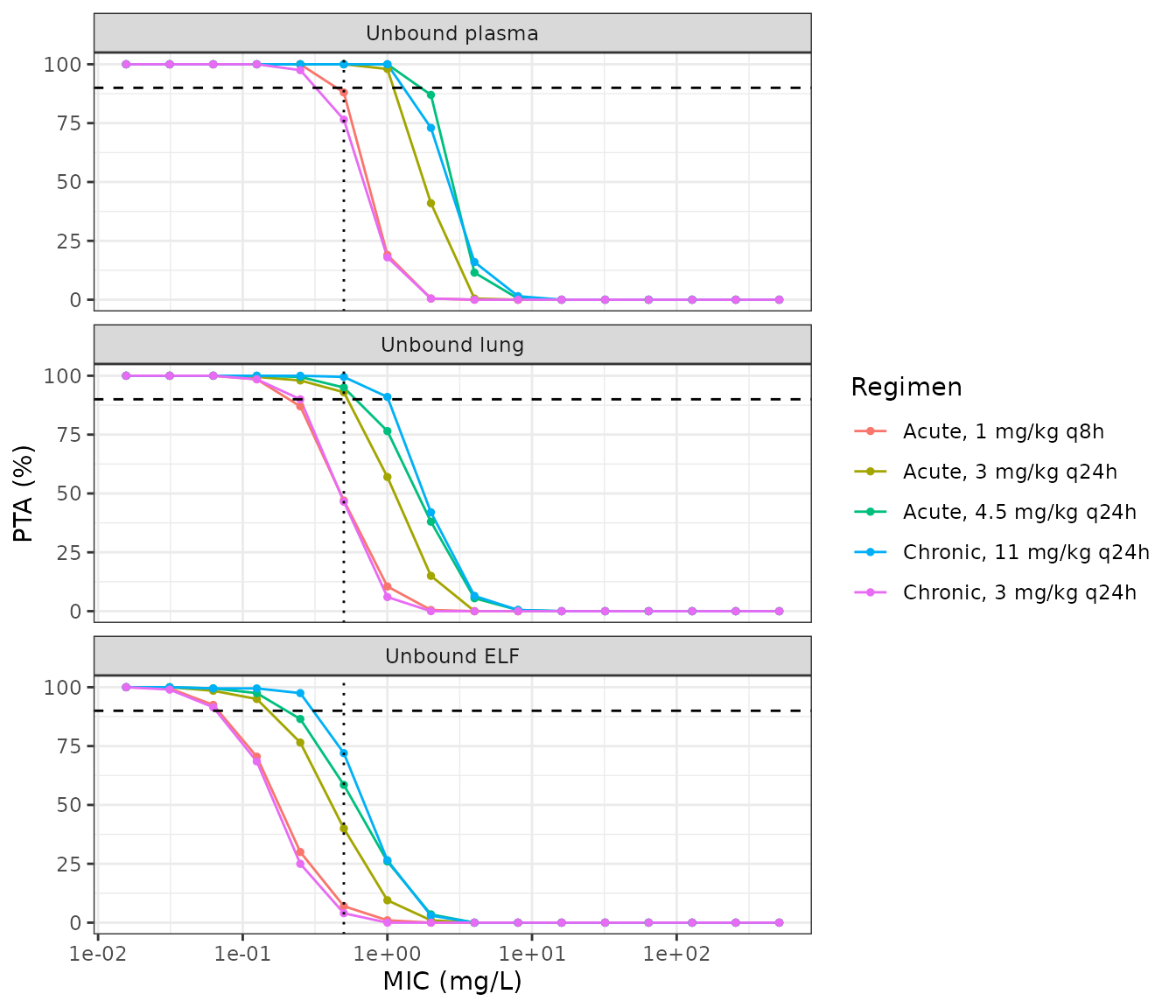
PTA across the EUCAST MIC range for each regimen and matrix (replicates Figure 3 of Dias 2022). The dashed line marks 90% PTA and the dotted line the modal MIC, 0.5 mg/L.
Assumptions and deviations
-
IIV scale. Table 1 reports IIV as %CV for
exponential random effects. The variances are
log(CV^2 + 1). The paper does not say whether its percentages are this log-normal CV or100 x omega. The other reading (variance = CV^2) changes the PTA in the table above by at most about 7 points, so the PTA comparison cannot tell the two apart. - Residual-error scale. Table 1 gives the log-additive errors (0.152 plasma, 0.313 microdialysis) without saying whether they are SDs or variances. They are encoded as SDs. As SDs they mean about 15% and 31% error, which is plausible for an LC-MS/MS plasma assay and for recovery-corrected microdialysate.
-
One microdialysis error, two endpoints. The paper
estimated a single log-additive error for all microdialysate data (lung
and ELF). nlmixr2 needs one residual parameter per endpoint, so the
estimate is carried twice (
expSd_Clung,expSd_Celf) with equal values. - Microdialysate collection intervals. The authors fitted microdialysate data as the integral over each 30-min collection interval. The packaged model returns the instantaneous unbound concentration. To fit interval data, average the prediction over each interval.
- Rat body weight for simulation. The paper simulates mg/kg doses but does not give the body weight used. The allometric scaling (Equation S2) used a 0.35 kg rat, while the study animals weighed 200-250 g. This page uses 0.25 kg, the top of the study range and a conventional reference rat weight. Both weights were tried. Parameters are absolute (L, L/h) because body weight was not retained as a covariate, so concentrations scale in direct proportion to the assumed weight. A 0.35 kg rat raises total-plasma PTA for the acute 1 mg/kg q8h regimen from about 90% to 99% (paper: 90%), so 0.25 kg also agrees better with the paper’s plasma results. No model parameter was changed.
-
ELF PTA at the high-exposure regimens. At acute 3
mg/kg q24h and chronic 11 mg/kg q24h, the simulated ELF PTA is two to
three times the published value (15.8% and 30.2%). The source does not
explain the gap. The ELF equation is printed explicitly as
(A3/V3) * Dfactor, and the lung PTA is close, so the implementation follows the printed model. A related point: the paper quotes an ELF/plasma penetration ratio of 13% for its simulated human-equivalent dose. That is lower than the peak ratio this implementation gives (about 25% unbound ELF to unbound plasma). The paper does not say how its ratio was computed or which group it used. - Comparison with Boselli 2007 (Supplementary Figure S8) is not reproduced. The paper gives neither the sampling times nor the infection group behind its simulated 32nd-68th percentile ranges.
- Covariate groups. The healthy, acute, chronic and blank-bead arms are mutually exclusive. Setting more than one indicator to 1 has no meaning in the source model.