Lumefantrine in severely malnourished children (Chotsiri 2019) • nlmixr2lib

Model and source

Citation: Chotsiri P, Denoeud-Ndam L, Baudin E, Guindo O, Diawara H, Attaher O, et al. (2019). Severe acute malnutrition results in lower lumefantrine exposure in children treated with artemether-lumefantrine for uncomplicated malaria. Clinical Pharmacology and Therapeutics 106(6):1299-1309. doi:10.1002/cpt.1531.
Article: https://doi.org/10.1002/cpt.1531
Trial: MAL-NUT, ClinicalTrials.gov https://clinicaltrials.gov/study/NCT01958905
Applying publication also reproduced here: Simeon S, Hughes E, Wallender E, Solans BP, Savic R (2024). Optimizing lumefantrine dosing for young children in high-malaria-burden countries using pharmacokinetic-pharmacodynamic simulations. Open Forum Infectious Diseases 11(11):ofae627. doi:10.1093/ofid/ofae627. https://doi.org/10.1093/ofid/ofae627

Simeon 2024 develops no model of its own: its Methods state that it “used a published LF PK-PD model from Chotsiri et al” and that simulations were run “using the Chotsiri et al model described above … sampled from the population parameter and variability distributions estimated by Chotsiri et al.” The model packaged here is therefore the Chotsiri 2019 model, and the final section of this vignette reproduces the Simeon 2024 dosing-regimen comparison with it.

mod_fn <- readModelDb("Chotsiri_2019_lumefantrine")
mod    <- rxode2::rxode2(mod_fn())
#> Warning: some etas defaulted to non-mu referenced, possible parsing error: etalfdepot
#> as a work-around try putting the mu-referenced expression on a simple line

The model has two endpoints: the lumefantrine capillary blood concentration Cc (ug/mL) and the reinfection-free survivor function sur (the probability of remaining free of P. falciparum reinfection). Both are algebraic outputs, so observation records carry cmt = NA_character_ and dvid = 1L, and rxode2 returns both as columns on every observation row.

Population

The model was built from the MAL-NUT trial (NCT01958905), an open comparative intervention study of artemether-lumefantrine conducted at Oulessebougou District Hospital (Koulikoro, Mali) and the primary healthcare centre of Andoume (Maradi City, Niger). Children aged 6-59 months with uncomplicated P. falciparum malaria were enrolled and classified as having severe acute malnutrition (SAM) per WHO criteria: weight-for-height z-score below -3 and/or mid-upper arm circumference (MUAC) below 115 mm. Children with kwashiorkor, severe stunting, severe anaemia, chronic disease, or complications requiring hospitalisation were excluded.

The pharmacokinetic analysis used 1,342 capillary dried-blood-spot concentrations from 131 SAM children (642 samples) and 160 non-SAM children (700 samples); 6.26% of samples fell below the 39.1 ng/mL limit of quantification and were handled by the M6 method. Five samples were drawn per child: one at a randomly allocated time among 6, 12, 24, 36 or 48 h, then at 60 h, 72 h, day 7, and either day 14 or day 21. The pharmacodynamic (time-to-reinfection) analysis pooled the PK-PD arm with a separate PD-only arm of 108 non-SAM children, giving 380 analysable children and 95 reinfections over 42 days of follow-up.

Baseline characteristics from Chotsiri 2019 Table 1, reported as median (95% CI):

Characteristic	SAM (n = 131)	Non-SAM (n = 160)
Age (months)	15 (6.3, 39)	27 (8.0, 53)
Body weight (kg)	6.78 (5.07, 10.5)	10.9 (6.84, 15.9)
MUAC (mm)	116 (104, 131)	140 (122, 163)
Weight-for-height z-score	-3.52 (-4.95, -2.60)	-1.07 (-2.58, 0.759)
Total lumefantrine dose (mg/kg)	105 (64.8, 142)	68.2 (48.3, 106)
Reinfections	34/131 (23.7%)	61/160 (38.1%)

The same information is available programmatically via readModelDb("Chotsiri_2019_lumefantrine")()$population.

Source trace

Every parameter and equation traces to Chotsiri 2019 or its supplementary methods; per-parameter source locations are also recorded inline next to each ini() entry in inst/modeldb/specificDrugs/Chotsiri_2019_lumefantrine.R.

Equation / parameter	Value	Source location
`lmtt = log(3.48)` (MTT, h)	3.48	Table 2 ‘MTT’ (RSE 11.7%; 95% CI 2.52-4.35)
`lcl = log(2.34)` (CL/F, L/h)	2.34	Table 2 ‘CL/F’ (RSE 6.25%; 95% CI 2.20-2.81)
`lvc = log(110)` (Vc/F, L)	110	Table 2 ‘VC/F’ (RSE 4.46%; 95% CI 101-123)
`lq = log(1.10)` (Q/F, L/h)	1.10	Table 2 ‘QP/F’ (RSE 8.10%; 95% CI 0.942-1.33)
`lvp = log(872)` (Vp/F, L)	872	Table 2 ‘VP/F’ (RSE 13.9%; 95% CI 635-1,200)
`lfdepot = fixed(log(1))` (F)	1 (fixed)	Table 2 ‘F 1 (fixed)’
`boxcox_fdepot = -0.373`	-0.373	Table 2 ‘Box-Cox on F’ (RSE 54.5%; 95% CI -0.742 to 0.205)
`e_wt_cl = fixed(0.75)`, `e_wt_vc = fixed(1)`	0.75 / 1.00 fixed	Supplementary methods: `theta_i = theta * exp(eta) * (BW_i / 9.62)^n`, n = 0.75 clearances, 1.00 volumes
`tm50_cl = 2.91` (months)	2.91	Table 2 ‘TM50’ (RSE 31.5%; 95% CI 2.86-5.98)
`hill_cl = fixed(1)`	1 (fixed)	Table 2 ‘alpha 1 (fixed)’; supplementary methods `MF = AGE^alpha / (TM50^alpha + AGE^alpha)`
`e_muac_f = -log(1 - 0.254)` per cm	25.4% per cm	Table 2 ‘MUAC on F (% per 1 cm)’ (RSE 5.24%; 95% CI 21.3-27.1%); Abstract ‘25.4% decreased absorption per 1 cm reduction’
`muac_ref = fixed(13.0)` (cm)	130 mm	Not reported; derived – see Assumptions and deviations
`dose50 = fixed(3.86)` (mg/kg)	3.86	Supplementary methods ‘In silico lumefantrine dose optimisation’; fixed from Kloprogge 2018 Table 2
`dose_std = fixed(120)` (mg)	120	Methods ‘Study design’: 1 tablet (120 mg lumefantrine) per dose below 15 kg
`lbase = log(5.25 / (365.25 * 24))` (1/h)	5.25 reinfections/year	Table 2 ‘BASE’ (RSE 11.8%; 95% CI 4.19-6.85)
`lic50 = log(0.156)` (ug/mL)	156 ng/mL	Table 2 ‘IC50’ (RSE 12.1%; 95% CI 141-214)
`lhill = log(4.77)`	4.77	Table 2 ‘gamma’ (RSE 38.8%; 95% CI 2.30-9.78)
`emax = fixed(1)`	1	Not reported; fixed – see Assumptions and deviations
`etalfdepot ~ 0.343306`	CV 64.0%	Table 2 ‘BSV F’ (RSE 7.08%); variance = log(0.640^2 + 1) per Table 2 footnote a
`etalmtt ~ 1.544665`	CV 192%	Table 2 ‘BSV MTT’ (RSE 8.88%); variance = log(1.92^2 + 1)
`etalq ~ 0.378220`	CV 67.8%	Table 2 ‘BSV QP/F’ (RSE 7.69%); variance = log(0.678^2 + 1)
`propSd = 0.582237`	sigma 0.339 (variance)	Table 2 ‘sigma’ (RSE 5.20; 95% CI 0.265-0.426); footnote defines sigma as the residual error variance, so SD = sqrt(0.339)
`addSd = 0.001`	–	Not from the source; placeholder residual on `sur` – see Assumptions and deviations
Two transit compartments, `ka = ktr = 3 / MTT`	–	Results ‘PK model’: ‘A transit-absorption model with two transit-compartments was superior’; supplementary methods: ‘the absorption constant (Ka) and transit rate constant (Ktr) were assumed to be equal’
Two-compartment disposition	–	Results ‘PK model’: two-compartment disposition (dOFV = -753 vs one-compartment)
Box-Cox IIV on F	–	Supplementary methods: `eta_transformed = ((exp(eta_F))^lambda - 1) / lambda`, `F_i = theta_F * exp(eta_transformed)` (Petersson 2009)
Additive error on log concentration -> proportional in nlmixr2	–	Supplementary methods: ‘additive error on the log-transformed observed concentrations (equivalent to an exponential error on an arithmetic scale)’
`LFEFF = 1 - Emax * Cp^gamma / (IC50^gamma + Cp^gamma)`	–	Supplementary methods, PD analysis
`Hz(t) = theta_BASE * LFEFF`; `S(t) = exp(-integral Hz dt)`	–	Supplementary methods, PD analysis (sign corrected – see Assumptions and deviations)
Dose-saturable F: `1 - Dosage / (Dose50 + Dosage)`	–	Supplementary methods, ‘In silico lumefantrine dose optimisation’ (normalised here – see Assumptions and deviations)

Typical-value profiles and validation against Table 3

Chotsiri 2019 Table 3 reports secondary parameters derived from the Bayesian post-hoc estimates of the final PK model. They are reproduced here with a typical-value (no random effects) simulation at each group’s median body weight, age and MUAC from Table 1, on the standard regimen of one 120 mg lumefantrine tablet every 12 h for 3 days.

obs_grid <- sort(unique(c(
  seq(0, 12, by = 0.25), seq(12.5, 72, by = 0.5),
  seq(73, 168, by = 1), seq(170, 336, by = 2), seq(340, 672, by = 4)
)))

build_events <- function(subjects, dose_times, obs_times) {
  out <- vector("list", nrow(subjects))
  for (i in seq_len(nrow(subjects))) {
    s <- subjects[i, ]
    dose_rows <- data.frame(
      id = s$id, time = dose_times, evid = 1L, amt = s$DOSE,
      cmt = "depot", dvid = NA_integer_
    )
    obs_rows <- data.frame(
      id = s$id, time = obs_times, evid = 0L, amt = NA_real_,
      cmt = NA_character_, dvid = 1L
    )
    rows <- rbind(dose_rows, obs_rows)
    rows$group   <- s$group
    rows$regimen <- s$regimen
    rows$WT      <- s$WT
    rows$PNA     <- s$PNA
    rows$MUAC    <- s$MUAC
    rows$DOSE    <- s$DOSE
    out[[i]] <- rows
  }
  ev <- dplyr::bind_rows(out)
  ev[order(ev$id, ev$time, -ev$evid), ]
}

typ_subj <- tibble::tibble(
  id      = 1:2,
  group   = c("SAM", "Non-SAM"),
  regimen = "standard",
  WT      = c(6.78, 10.9),   # Table 1 median body weight
  PNA     = c(15, 27),       # Table 1 median age (months)
  MUAC    = c(116, 140),     # Table 1 median MUAC (mm)
  DOSE    = 120
)

typ_events <- build_events(typ_subj, dose_times = seq(0, 60, by = 12),
                           obs_times = obs_grid)

sim_typ <- rxode2::rxSolve(
  mod, events = typ_events, omega = NA,
  keep = c("group", "regimen", "WT", "PNA", "MUAC", "DOSE")
) |>
  as.data.frame()
#> Warning: multi-subject simulation without without 'omega'
stopifnot(!anyNA(sim_typ$Cc), all(sim_typ$Cc >= 0))

ggplot(sim_typ, aes(time / 24, Cc * 1000, colour = group)) +
  geom_line(linewidth = 0.7) +
  geom_hline(yintercept = c(164, 182), linetype = "dotted", colour = "grey40") +
  geom_hline(yintercept = 200, linetype = "dashed", colour = "grey40") +
  scale_y_log10() +
  labs(x = "Days after first dose", y = "Lumefantrine (ng/mL)", colour = NULL,
       title = "Typical-value lumefantrine profiles, standard regimen",
       caption = paste(
         "Typical child at each group's Table 1 median weight, age and MUAC.",
         "Dashed line: 200 ng/mL day-7 efficacy threshold. Dotted band:",
         "clinical MIC 164-182 ng/mL (Chotsiri 2019 Results)."
       ))
#> Warning in scale_y_log10(): log-10 transformation introduced infinite values.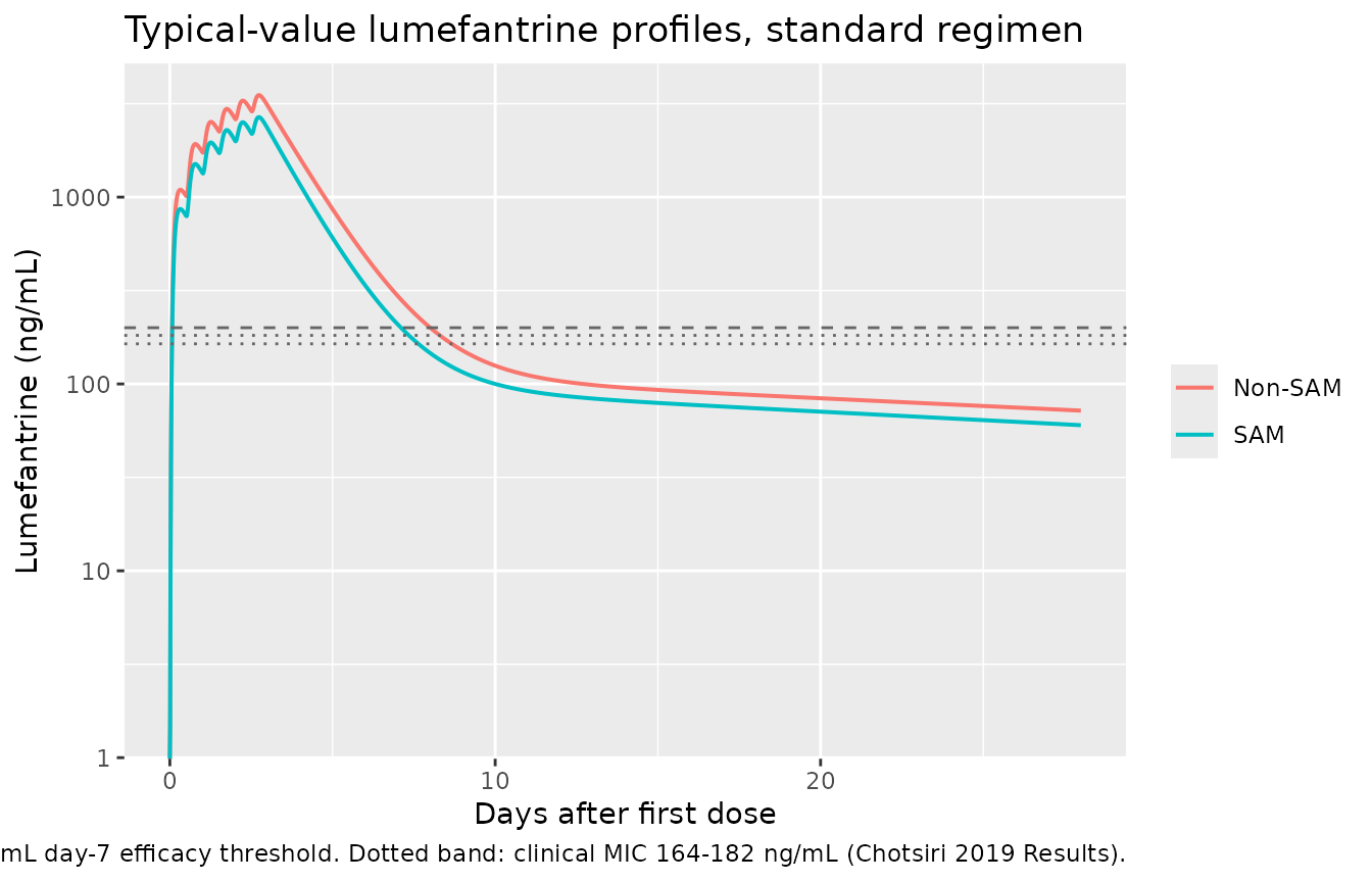

PKNCA on the typical-value profiles

nca_conc <- sim_typ |>
  dplyr::filter(!is.na(Cc)) |>
  dplyr::mutate(conc_ng_mL = Cc * 1000) |>
  dplyr::select(id, group, time, conc_ng_mL)

nca_dose <- typ_events |>
  dplyr::filter(evid == 1) |>
  dplyr::select(id, group, time, amt)

conc_obj <- PKNCA::PKNCAconc(nca_conc, conc_ng_mL ~ time | group + id,
                             concu = "ng/mL", timeu = "h")
dose_obj <- PKNCA::PKNCAdose(nca_dose, amt ~ time | group + id, doseu = "mg")

intervals <- data.frame(
  start = 0, end = 672,
  cmax = TRUE, tmax = TRUE, auclast = TRUE, half.life = TRUE
)

nca_res <- PKNCA::pk.nca(PKNCA::PKNCAdata(conc_obj, dose_obj,
                                          intervals = intervals))
nca_df <- as.data.frame(nca_res$result)

Chotsiri 2019 reports Tmax relative to the last dose: the tabulated 5.69 h plus the 60 h last-dose time equals the time of the overall peak concentration. The simulated tmax is therefore shifted by the last dose time before comparison, and the day-7 concentration is read directly off the profile.

day7 <- sim_typ |>
  dplyr::filter(abs(time - 168) < 1e-6) |>
  dplyr::transmute(group, PPTESTCD = "cday7", PPORRES = Cc * 1000)

sim_nca <- nca_df |>
  dplyr::filter(PPTESTCD %in% c("cmax", "tmax", "auclast", "half.life")) |>
  dplyr::mutate(
    PPORRES = dplyr::case_when(
      PPTESTCD == "tmax"    ~ PPORRES - 60,     # relative to the last dose
      PPTESTCD == "auclast" ~ PPORRES / 1000,   # ng*h/mL -> h*ug/mL
      PPTESTCD == "half.life" ~ PPORRES / 24,   # h -> days
      TRUE ~ PPORRES
    )
  ) |>
  dplyr::select(group, PPTESTCD, PPORRES) |>
  dplyr::bind_rows(day7)

# Chotsiri 2019 Table 3, median values
ref_nca <- data.frame(
  group     = c("SAM", "Non-SAM"),
  cmax      = c(2900, 3360),
  tmax      = c(5.69, 5.69),
  half.life = c(3.10, 3.54),
  cday7     = c(222, 300),
  auclast   = c(262, 316)
)

nca_tbl <- nlmixr2lib::ncaComparisonTable(
  sim_nca, ref_nca, by = "group",
  units = c(cmax = "ng/mL", tmax = "h", half.life = "days",
            cday7 = "ng/mL", auclast = "h*ug/mL")
)
#> Warning: ncaParamLabel(): unknown PKNCA code(s) returned as-is: 'cday7'
# `cday7` is not a PKNCA code, so it is passed through unlabelled.
nca_tbl[[1]] <- sub("^cday7 ", "Day-7 conc ", nca_tbl[[1]])

knitr::kable(
  nca_tbl,
  caption = paste(
    "Typical-value simulation vs Chotsiri 2019 Table 3 secondary parameter",
    "medians. AUC is the 0-28 day AUC; cday7 is the day-7 concentration."
  ),
  digits = 2
)

Typical-value simulation vs Chotsiri 2019 Table 3 secondary parameter medians. AUC is the 0-28 day AUC; cday7 is the day-7 concentration.
NCA parameter	group	Reference	Simulated	% diff
Cmax (ng/mL)	SAM	2900	2680	-7.6%
Cmax (ng/mL)	Non-SAM	3360	3510	+4.6%
Tmax (h)	SAM	5.69	5.5	-3.3%
Tmax (h)	Non-SAM	5.69	5.5	-3.3%
AUClast (h*ug/mL)	SAM	262	248	-5.5%
AUClast (h*ug/mL)	Non-SAM	316	325	+2.9%
t½ (days)	SAM	3.1	33	+964.4%*
t½ (days)	Non-SAM	3.54	36.1	+919.3%*
Day-7 conc (ng/mL)	SAM	222	209	-5.9%
Day-7 conc (ng/mL)	Non-SAM	300	296	-1.2%

attr(nca_tbl, "footnote")
#> [1] "* differs from reference by more than ±20%."

Four of the five parameters – Cmax, Tmax, day-7 concentration and AUC(0-28 d) – agree with the published medians to within about 8% in both groups, which is the level of agreement achievable given that Table 3 summarises post-hoc estimates across each whole group rather than a single typical child.

The terminal half-life is the exception and is flagged. The reason is structural rather than an encoding error: with Vp/F = 872 L and Q/F = 1.10 L/h, the model’s true terminal phase is very slow and very low in amplitude.

# Fit on a uniform 6-hourly grid inside each window: an unweighted
# log-linear fit over a graded observation grid would otherwise depend on
# how densely each part of the window happens to be sampled.
half_life_windows <- function(dat) {
  vapply(list(c(72, 336), c(72, 504)), function(w) {
    tt <- seq(w[1], w[2], by = 6)
    cc <- stats::approx(dat$time, dat$Cc * 1000, xout = tt)$y
    unname(log(2) / -coef(stats::lm(log(cc) ~ tt))[2] / 24)
  }, numeric(1))
}
hl <- sim_typ |>
  dplyr::group_by(group) |>
  dplyr::group_modify(~ {
    v <- half_life_windows(.x)
    tibble::tibble(`Apparent t1/2, day 3-14 (d)` = v[1],
                   `Apparent t1/2, day 3-21 (d)` = v[2])
  }) |>
  dplyr::ungroup() |>
  dplyr::mutate(`Published t1/2 (d)` = c(3.54, 3.10)) |>
  dplyr::rename(Group = group)
knitr::kable(hl, digits = 2, caption = paste(
  "Apparent half-life from a log-linear fit over two windows inside the",
  "trial's sampling range, compared with the published value."
))

Apparent half-life from a log-linear fit over two windows inside the trial’s sampling range, compared with the published value.
Group	Apparent t1/2, day 3-14 (d)	Apparent t1/2, day 3-21 (d)	Published t1/2 (d)
Non-SAM	2.25	4.33	3.54
SAM	2.41	4.71	3.10

The published 3.10 and 3.54 day half-lives fall between the apparent half-lives fitted over day 3-14 and over day 3-21, i.e. they are of the magnitude produced by a slope estimated over the interval the trial actually sampled (last samples at day 7 and day 14 or 21). They are not the model’s structural terminal half-life, which this sampling design could not resolve.

Two caveats on this comparison. First, an apparent half-life is not a well-defined property of the model: its value depends on the fitting window (and, if the fit is unweighted, on the observation density within it), so the numbers above should be read as a magnitude check rather than a match. Running PKNCA’s own terminal-slope selection over the trial’s actual sampling times instead gives about 8 to 9 days. Second, the model orders the two groups the other way round from the paper: it gives a slightly longer apparent half-life in SAM children, whereas Table 3 reports a shorter one (3.10 vs 3.54 days, p = 0.0006). In the model, SAM children are both lighter (which shortens half-life through V/CL scaling as WT^0.25) and younger (which lengthens it through reduced maturation of CL/F), and the maturation term slightly dominates. No parameter was adjusted to remove either discrepancy.

Time above the clinical MIC

Chotsiri 2019 reports a further quantity that is independent of Table 3 and that tests the absolute concentration scale rather than the ratio between groups: time above the clinical minimum inhibitory concentration after standard dosing, 8.05 days in SAM and 9.33 days in non-SAM children, against an estimated clinical MIC of 164 to 182 ng/mL.

published_tmic <- data.frame(
  group = c("SAM", "Non-SAM"),
  `Published t > MIC (days)` = c(8.05, 9.33),
  check.names = FALSE
)

tam <- sim_typ |>
  dplyr::group_by(group) |>
  dplyr::summarise(
    `Simulated t > MIC (days)` = max(time[Cc * 1000 >= 164]) / 24,
    .groups = "drop"
  ) |>
  dplyr::left_join(published_tmic, by = "group") |>
  dplyr::rename(Group = group)

knitr::kable(tam, digits = 2, caption = paste(
  "Time above the lower bound of the clinical MIC band (164 ng/mL) after",
  "the standard regimen, compared with Chotsiri 2019 Results."
))

Time above the lower bound of the clinical MIC band (164 ng/mL) after the standard regimen, compared with Chotsiri 2019 Results.
Group	Simulated t > MIC (days)	Published t > MIC (days)
Non-SAM	8.58	9.33
SAM	7.58	8.05

This is the most direct check on the derived MUAC centering value, because it depends on where the concentration-time curve sits in absolute terms rather than on the SAM/non-SAM contrast. Both groups agree with the published values to within about 8%.

Virtual cohort and dosing regimens

For the regimen comparisons, Chotsiri 2019 simulated 1,000 hypothetical SAM and 1,000 hypothetical non-SAM children with body weight, age and MUAC “assumed to be uniformly distributed according to the observed value (Table 1)”. The same construction is used here at a smaller cohort size.

set.seed(20260810L)
n_per_arm <- 100L

groups <- tibble::tribble(
  ~group,    ~wt_lo, ~wt_hi, ~pna_lo, ~pna_hi, ~muac_lo, ~muac_hi,
  "SAM",       5.07,   10.5,     6.3,      39,      104,      131,
  "Non-SAM",   6.84,   15.9,     8.0,      53,      122,      163
)

regimens <- tibble::tribble(
  ~regimen,      ~extra_tablets, ~interval_h, ~n_doses,
  "standard",                0L,          12,       6L,
  "increased",               1L,          12,       6L,
  "intensified",             0L,           8,       9L,
  "extended",                0L,          12,      10L
)

who_tablets <- function(wt) ifelse(wt < 15, 1L, 2L)

cohort <- dplyr::bind_rows(lapply(seq_len(nrow(groups)), function(g) {
  gr <- groups[g, ]
  tibble::tibble(
    group = gr$group,
    WT    = runif(n_per_arm, gr$wt_lo,   gr$wt_hi),
    PNA   = runif(n_per_arm, gr$pna_lo,  gr$pna_hi),
    MUAC  = runif(n_per_arm, gr$muac_lo, gr$muac_hi)
  )
}))

arms <- tidyr::crossing(cohort, regimens) |>
  dplyr::mutate(
    id   = dplyr::row_number(),
    DOSE = (who_tablets(WT) + extra_tablets) * 120
  )

The four regimens are those of Chotsiri 2019 supplementary methods and Simeon 2024 Table 2: standard (WHO-recommended, twice daily for 3 days), increased (one extra 120 mg tablet per dose), intensified (thrice daily for 3 days) and extended (twice daily for 5 days).

pd_grid <- sort(unique(c(
  seq(0, 12, by = 0.5), seq(13, 72, by = 1), seq(74, 168, by = 2),
  seq(172, 336, by = 4), seq(348, 1008, by = 12)
)))

arm_events <- dplyr::bind_rows(lapply(seq_len(nrow(arms)), function(i) {
  s <- arms[i, ]
  build_events(
    dplyr::mutate(s, regimen = s$regimen),
    dose_times = seq(0, by = s$interval_h, length.out = s$n_doses),
    obs_times  = pd_grid
  )
}))

sim_arms <- rxode2::rxSolve(
  mod, events = arm_events,
  keep = c("group", "regimen", "WT", "PNA", "MUAC", "DOSE")
) |>
  as.data.frame() |>
  dplyr::mutate(
    regimen = factor(regimen,
                     levels = c("standard", "increased", "intensified", "extended"))
  )
stopifnot(!anyNA(sim_arms$Cc), all(sim_arms$Cc >= 0), all(sim_arms$sur <= 1))

Replicate Figure 4: exposure by dosing regimen

Chotsiri 2019 Figure 4 plots predicted day-7 concentration, AUC and Cmax for SAM and non-SAM children under each regimen.

exposure <- sim_arms |>
  dplyr::group_by(id, group, regimen) |>
  dplyr::summarise(
    day7 = Cc[which.min(abs(time - 168))] * 1000,
    cmax = max(Cc, na.rm = TRUE) * 1000,
    .groups = "drop"
  )

exposure |>
  tidyr::pivot_longer(c(day7, cmax), names_to = "metric", values_to = "value") |>
  dplyr::mutate(metric = factor(metric, c("day7", "cmax"),
                                c("Day-7 concentration", "Cmax"))) |>
  ggplot(aes(regimen, value, fill = group)) +
  geom_boxplot(outlier.size = 0.5, coef = 0) +
  facet_wrap(~metric, scales = "free_y") +
  scale_y_log10() +
  theme(axis.text.x = element_text(angle = 30, hjust = 1)) +
  labs(x = NULL, y = "Lumefantrine (ng/mL)", fill = NULL,
       title = "Replicates Chotsiri 2019 Figure 4 (panels a and c)",
       caption = paste(
         "Boxes 25-75% with median; whiskers suppressed. n =", n_per_arm,
         "per group per regimen. Covariates uniform over the Table 1 ranges."
       ))

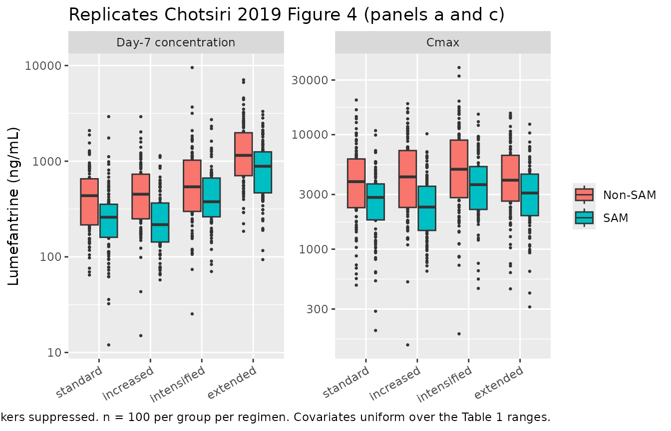
Consistent with the paper, the increased regimen barely improves exposure – the extra tablet is largely offset by dose-limited absorption – while the intensified and especially the extended regimens raise SAM exposure toward that of non-SAM children on standard dosing.

Replicate Table S1: malaria-free incidence by regimen

Chotsiri 2019 Table S1 reports the simulated proportion of children remaining malaria free at day 20 and day 42. The model’s survivor output sur gives the per-child probability of remaining reinfection free, so the population proportion is its mean across the cohort.

mf <- sim_arms |>
  dplyr::filter(time %in% c(20 * 24, 42 * 24)) |>
  dplyr::mutate(day = paste0("Day ", time / 24)) |>
  dplyr::group_by(group, regimen, day) |>
  dplyr::summarise(Simulated = 100 * mean(sur), .groups = "drop")

ref_s1 <- tibble::tribble(
  ~group,     ~regimen,      ~day,     ~Published,
  "SAM",      "standard",    "Day 20", 87.5,
  "SAM",      "increased",   "Day 20", 88.5,
  "SAM",      "intensified", "Day 20", 91.0,
  "SAM",      "extended",    "Day 20", 93.5,
  "Non-SAM",  "standard",    "Day 20", 90.0,
  "Non-SAM",  "increased",   "Day 20", 91.0,
  "Non-SAM",  "intensified", "Day 20", 93.5,
  "Non-SAM",  "extended",    "Day 20", 95.0,
  "SAM",      "standard",    "Day 42", 64.5,
  "SAM",      "increased",   "Day 42", 65.0,
  "SAM",      "intensified", "Day 42", 69.5,
  "SAM",      "extended",    "Day 42", 72.5,
  "Non-SAM",  "standard",    "Day 42", 67.3,
  "Non-SAM",  "increased",   "Day 42", 69.5,
  "Non-SAM",  "intensified", "Day 42", 74.0,
  "Non-SAM",  "extended",    "Day 42", 77.0
) |>
  dplyr::mutate(regimen = factor(regimen, levels = levels(sim_arms$regimen)))

s1 <- dplyr::left_join(ref_s1, mf, by = c("group", "regimen", "day")) |>
  dplyr::mutate(`Difference (pp)` = Simulated - Published) |>
  dplyr::arrange(day, group, regimen) |>
  dplyr::rename(Group = group, Regimen = regimen, Day = day,
                `Published (%)` = Published, `Simulated (%)` = Simulated)

knitr::kable(s1, digits = 1, caption = paste(
  "Malaria-free incidence: Chotsiri 2019 Table S1 vs this model.",
  "Published values are medians of 100 simulation replicates; simulated",
  "values are the mean survivor probability across", n_per_arm,
  "children per arm."
))

Malaria-free incidence: Chotsiri 2019 Table S1 vs this model. Published values are medians of 100 simulation replicates; simulated values are the mean survivor probability across 100 children per arm.
Group	Regimen	Day	Published (%)	Simulated (%)	Difference (pp)
Non-SAM	standard	Day 20	90.0	89.8	-0.2
Non-SAM	increased	Day 20	91.0	90.1	-0.9
Non-SAM	intensified	Day 20	93.5	91.9	-1.6
Non-SAM	extended	Day 20	95.0	94.0	-1.0
SAM	standard	Day 20	87.5	87.0	-0.5
SAM	increased	Day 20	88.5	86.1	-2.4
SAM	intensified	Day 20	91.0	89.8	-1.2
SAM	extended	Day 20	93.5	92.0	-1.5
Non-SAM	standard	Day 42	67.3	70.8	3.5
Non-SAM	increased	Day 42	69.5	70.9	1.4
Non-SAM	intensified	Day 42	74.0	75.8	1.8
Non-SAM	extended	Day 42	77.0	78.5	1.5
SAM	standard	Day 42	64.5	65.8	1.3
SAM	increased	Day 42	65.0	64.4	-0.6
SAM	intensified	Day 42	69.5	70.0	0.5
SAM	extended	Day 42	72.5	73.2	0.7

sim_arms |>
  dplyr::group_by(group, regimen, time) |>
  dplyr::summarise(mf = 100 * mean(sur), .groups = "drop") |>
  dplyr::filter(time <= 42 * 24) |>
  ggplot(aes(time / 24, mf, colour = regimen)) +
  geom_line(linewidth = 0.7) +
  facet_wrap(~group) +
  labs(x = "Days after first dose", y = "Malaria free (%)", colour = NULL,
       title = "Replicates Chotsiri 2019 Figure S5",
       caption = "Mean survivor probability over the 42-day follow-up.")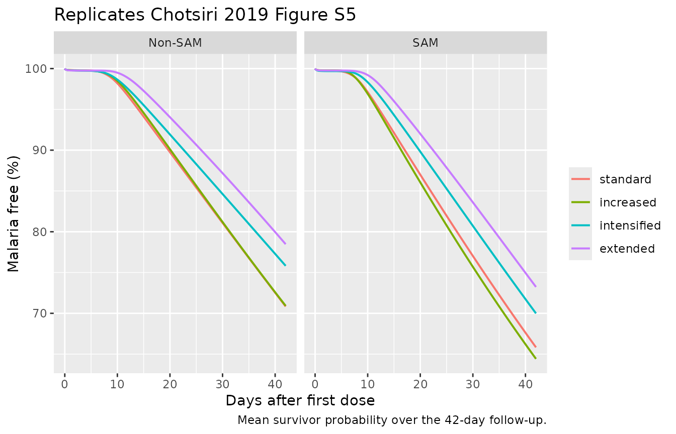

Reproducing Simeon 2024

Simeon 2024 applied this model to 372,363 children under 5 from Demographic and Health Surveys data in 25 high-malaria-burden countries, evaluating (i) the proportion reaching a day-7 lumefantrine concentration of at least 200 ng/mL and (ii) the proportion remaining malaria free for 42 days, under the same four regimens.

simeon <- exposure |>
  dplyr::left_join(
    sim_arms |>
      dplyr::filter(time == 42 * 24) |>
      dplyr::select(id, sur),
    by = "id"
  ) |>
  dplyr::group_by(group, regimen) |>
  dplyr::summarise(
    `Day-7 >= 200 ng/mL (%)` = 100 * mean(day7 >= 200),
    `Malaria free at day 42 (%)` = 100 * mean(sur),
    .groups = "drop"
  ) |>
  dplyr::rename(Group = group, Regimen = regimen)

knitr::kable(simeon, digits = 1, caption = paste(
  "Target attainment by regimen. Simeon 2024 reports, for the whole DHS",
  "population under WHO-method dosing, 74.6% (standard), 77.8% (increased)",
  "and 96.1% (extended) reaching 200 ng/mL, and 76.7% (standard) /",
  "82.0% (extended) malaria free at day 42."
))

Target attainment by regimen. Simeon 2024 reports, for the whole DHS population under WHO-method dosing, 74.6% (standard), 77.8% (increased) and 96.1% (extended) reaching 200 ng/mL, and 76.7% (standard) / 82.0% (extended) malaria free at day 42.
Group	Regimen	Day-7 >= 200 ng/mL (%)	Malaria free at day 42 (%)
Non-SAM	standard	78	70.8
Non-SAM	increased	80	70.9
Non-SAM	intensified	87	75.8
Non-SAM	extended	99	78.5
SAM	standard	66	65.8
SAM	increased	55	64.4
SAM	intensified	83	70.0
SAM	extended	95	73.2

The ordering Simeon 2024 reports is reproduced: the increased regimen gives almost no gain over standard because of absorption saturation, the intensified regimen gives a moderate gain, and the extended regimen gives the largest gain. The absolute percentages are not expected to match, because this cohort is the Chotsiri 2019 trial population (a malaria-treatment cohort split into SAM and non-SAM halves) rather than the DHS population Simeon simulated; see Assumptions and deviations.

The weight-band mechanism behind the ALT dosing method

Simeon 2024’s alternative (“ALT”) dosing method gives children with a weight-for-age z-score below 0 the WHO dose for their expected weight rather than their actual weight. Because the WHO rule is a step function of weight (1 tablet below 15 kg, 2 tablets for 15-25 kg), the method’s effect is concentrated in children whose expected weight crosses a band boundary; Simeon 2024 attributes its benefit to exactly this, noting that “children in the age band 36-59 months straddle between 2 LF dosing levels because of their varying weight around 15 kg”.

That mechanism is shown directly below by re-dosing the underweight children at the next weight band up, holding everything else fixed.

alt_subj <- arms |>
  dplyr::filter(regimen == "standard", group == "SAM") |>
  dplyr::mutate(id = id + 100000L, DOSE = (who_tablets(WT) + 1L) * 120,
                regimen = "standard")

alt_events <- dplyr::bind_rows(lapply(seq_len(nrow(alt_subj)), function(i) {
  build_events(alt_subj[i, ], dose_times = seq(0, 60, by = 12),
               obs_times = c(pd_grid))
}))

sim_alt <- rxode2::rxSolve(
  mod, events = alt_events,
  keep = c("group", "regimen", "WT", "PNA", "MUAC", "DOSE")
) |>
  as.data.frame()

alt_cmp <- dplyr::bind_rows(
  exposure |>
    dplyr::filter(group == "SAM", regimen == "standard") |>
    dplyr::transmute(method = "WHO method (actual weight)", day7),
  sim_alt |>
    dplyr::filter(abs(time - 168) < 1e-6) |>
    dplyr::transmute(method = "ALT method (next weight band)", day7 = Cc * 1000)
) |>
  dplyr::group_by(method) |>
  dplyr::summarise(
    `Median day-7 (ng/mL)` = median(day7),
    `Reaching 200 ng/mL (%)` = 100 * mean(day7 >= 200),
    .groups = "drop"
  ) |>
  dplyr::rename(`Dosing method` = method)

knitr::kable(alt_cmp, digits = 1, caption = paste(
  "Weight-band uplift in the SAM cohort on the standard regimen:",
  "the mechanism underlying Simeon 2024's ALT dosing method."
))

Weight-band uplift in the SAM cohort on the standard regimen: the mechanism underlying Simeon 2024’s ALT dosing method.
Dosing method	Median day-7 (ng/mL)	Reaching 200 ng/mL (%)
ALT method (next weight band)	213.1	54
WHO method (actual weight)	259.5	66

Assumptions and deviations

MUAC centering value (muac_ref = 13.0 cm) is not reported by the source. Chotsiri 2019 states the MUAC effect as “25.4% per 1 cm” but never gives the MUAC at which the effect is null. This matters: because theta_F is fixed to 1, the centering value alone sets the absolute scale of relative bioavailability, and hence of every predicted concentration – a 1 cm shift moves all concentrations by 29%. Two independent derivations agree on 130 mm. (a) It is the pooled central MUAC of the PK population: 129.1 mm as the group-size-weighted mean of the Denoeud-Ndam 2016 Table 1 group means, and about 131 mm from the pooled-median position implied by the Chotsiri Table 1 group medians (116 and 140 mm) and group sizes (131 and 160). This mirrors the paper’s own centering of the allometry on the pooled median body weight of 9.62 kg. (b) Back-solving from Table 3: requiring the model to reproduce each group’s published median AUC(0-28 d), and independently its published median day-7 concentration, at that group’s median weight, age and MUAC gives 128 mm from the SAM rows and 130 mm from the non-SAM rows. 13.0 cm is adopted as the rounded standard. Users with access to the original NONMEM control stream are encouraged to confirm this and file an erratum.
The functional form of the MUAC effect is inferred. The source prints no covariate equation for MUAC. An exponential (constant proportional) effect is used because the paper states the effect as a single “% per 1 cm” figure applied across the whole MUAC range in both the final model (25.4%) and the full covariate model (21.0%), which is only self-consistent for a constant proportional effect; because it keeps F strictly positive across the observed 104-163 mm range; and because it matches the multiplicative form used for the other covariates in this model family. A linear form gives numerically similar predictions over the observed range and is not excluded by any published quantity.
The dose-saturation term is normalised; the source prints it un-normalised. Chotsiri 2019 did not estimate the saturation term. It was added to the final model only for the dose-optimisation simulations, with Dose50 fixed at 3.86 mg/kg from Kloprogge 2018. Because it was bolted on after estimation, CL/F and Vc/F already absorb the standard-dose bioavailability, so applying the printed form F = theta_F * (1 - Dosage / (Dose50 + Dosage)) literally would multiply every predicted concentration by 0.236 at the standard dose – which is contradicted by the paper’s own Table 3, by Figure 4, and by its reported time above MIC of 8.05 days. The term is therefore normalised to each child’s standard 120 mg per-dose exposure, making it exactly inert on the standard regimen and active only at other dose levels. The normalisation cancels in every dose ratio, so the published dose comparison is untouched: for the typical 9.62 kg child, doubling the dose multiplies F by 0.567, matching the “43% decrease in bioavailability” that Simeon 2024 attributes to this model.
The survivor-function equation is sign-corrected. The supplementary methods print S(t) = exp(integral_0^t Hz(t) dt), which exceeds 1 for all t > 0 and is not a survivor function. The standard form S(t) = exp(-integral_0^t Hz(t) dt) is used. The supplement also prints I_start and I_end with the same divisor of 10^4 although the text states that I_end corresponds to 10^5 parasites; this affects only the interval-censoring likelihood used during estimation, not forward simulation, and is not encoded.
Emax is not reported and is fixed to 1. No value for Emax appears in Chotsiri 2019 or its supplement. It is fixed to 1, the only value consistent with the published parameterisation: the protective effect then spans 1 (no drug) to 0 (saturating concentrations), and IC50 is, as the supplement defines it, “the lumefantrine capillary blood concentration needed in order to reduce the hazard of malaria reinfection by 50%”.
sigma is read as a variance. The Table 2 footnote defines the tabulated quantity as “sigma, residual error variance of lumefantrine concentrations”, so the reported 0.339 is squared and the log-scale residual SD is sqrt(0.339) = 0.582. Note that the sibling Kloprogge 2018 model reports a numerically similar sigma = 0.323 whose own footnote calls it an “additive residual error on log scale” (i.e. a standard deviation); the two papers’ conventions differ, and this model follows its own paper’s footnote.
Placeholder residual on the survival endpoint. The source pharmacodynamic model is an interval-censored time-to-event likelihood, not an additively-observed continuous endpoint. sur is exposed as a second endpoint with a small placeholder additive residual (addSd = 0.001) purely so the nlmixr2 endpoint machinery accepts it; the value is not from the source and should not be used as an estimate of observation error. The same convention is used in Lindauer_2017_lacosamide_seizure.
Interindividual variability on CL/F, Vc/F and Vp/F is absent by design. Chotsiri 2019 estimated these close to zero and removed them from the final model, so simulated between-child variability in exposure comes from the Box-Cox IIV on F (CV 64%), the IIV on MTT (CV 192%) and on Q/F (CV 67.8%) alone.
Covariates are drawn independently and uniformly. Following the source’s own simulation design (“body-weight, age, and MUAC … assumed to be uniformly distributed according to the observed value”), the virtual cohort draws the three covariates independently over their Table 1 95% CI ranges. This discards the strong real correlation among weight, age and MUAC (Chotsiri 2019 Figure S2) and, because the observed distributions are right-skewed, shifts cohort medians relative to the published group medians. The Table 3 validation above therefore uses a typical-value simulation at the published median covariates rather than the cohort.
Cohort size. Chotsiri 2019 simulated 1,000 children per group and Simeon 2024 simulated 372,363; this vignette uses 100 per group per regimen to keep the render fast. Percentages therefore carry Monte Carlo noise of a few points.
Simeon 2024’s DHS cohort and WHO growth standards are not reproduced. Simeon 2024’s absolute target-attainment percentages depend on the Demographic and Health Surveys anthropometric extract for 25 countries, on its imputation of MUAC from the Chotsiri data, and on WHO Child Growth Standard charts used to derive expected weight for age. None of those data ship with this package, so the ALT method is demonstrated here through its operative mechanism (a weight-band uplift for underweight children) rather than reproduced numerically. The regimen ordering and the saturation-driven failure of the increased regimen do reproduce.
Artemether and desbutyl-lumefantrine are not modelled. The trial administered artemether-lumefantrine, but only lumefantrine was measured and modelled; the metabolite desbutyl-lumefantrine was not measured (Discussion). Companion artemether models in this package include modellib("Hoglund_2015_artemether") and modellib("Mosha_2014_artemether").
Concentrations are capillary blood. Samples were capillary dried blood spots measured by LC-MS/MS. Capillary and venous lumefantrine concentrations are highly correlated, but users comparing against venous-plasma models (such as Kloprogge_2018_lumefantrine) should apply an appropriate matrix correction.