Lopinavir + ritonavir + rifampicin DDI in adults and children (Zhang 2013)
Source:vignettes/articles/Zhang_2013_lopinavir_ritonavir.Rmd
Zhang_2013_lopinavir_ritonavir.Rmd
library(nlmixr2lib)
library(rxode2)
#> rxode2 5.1.2 using 2 threads (see ?getRxThreads)
#>   no cache: create with `rxCreateCache()`
library(dplyr)
#>
#> Attaching package: 'dplyr'
#> The following objects are masked from 'package:stats':
#>
#>     filter, lag
#> The following objects are masked from 'package:base':
#>
#>     intersect, setdiff, setequal, union
library(tidyr)
library(ggplot2)
library(PKNCA)
#>
#> Attaching package: 'PKNCA'
#> The following object is masked from 'package:stats':
#>
#>     filter
Lopinavir + ritonavir + rifampicin DDI model (Zhang 2013)
Replicate the integrated population pharmacokinetic model reported by Zhang et al. (2013) for lopinavir and ritonavir co-administered to HIV-infected adults and children with and without rifampicin-based antitubercular treatment. The model describes:
lopinavir as a 1-compartment first-order absorption substrate;
ritonavir as a 2-compartment substrate with a 2-transit-compartment absorption chain;
a sigmoidal-Emax inhibition of lopinavir apparent clearance by ritonavir plasma concentration (Emax = 0.82, EC50 = 0.098 mg/L, Hill = 2.8);
per-population (adult / child) rifampicin shifts on apparent clearance and bioavailability of both drugs;
a linear ritonavir-dose effect on relative bioavailability that drives the per-cohort differences across the standard / super-boosted / doubled-dose LPV/r regimens evaluated in the paper;
a step diurnal effect on apparent clearance (overnight reduction by 51% in adults / 27% in children) and on lopinavir bioavailability at the evening dose (+19% in adults; not supported in children or in the ritonavir output).
Citation: Zhang C, Denti P, Decloedt EH, Ren Y, Karlsson MO, McIlleron H. Model-based evaluation of the pharmacokinetic differences between adults and children for lopinavir and ritonavir in combination with rifampicin. Br J Clin Pharmacol. 2013;76(5):741-751. doi:10.1111/bcp.12101.
Article: https://doi.org/10.1111/bcp.12101
Population
The Zhang 2013 cohort pools three previously reported South African studies (Zhang 2013 Methods, refs 3 / 5 / 6 and Table 1): 21 HIV-infected adult volunteers (median age 36 years, range 26-58; median body weight 64.5 kg, range 43-110; 18 of 21 female) virologically suppressed on LPV/r 400/100 mg 12-hourly plus two NRTIs; 39 HIV-infected children without tuberculosis on the standard 230/57.5 mg/m^2 12-hourly LPV/r oral solution (median age 21 months, range 6 months-4.5 years; median weight 10.2 kg, range 5.0-17.0; median LPV dose 11.6 mg/kg, range 9.2-16.0); and 35 HIV-infected children with active tuberculosis on rifampicin-based antitubercular therapy, of whom 15 received the ‘super-boosted’ regimen (LPV : RTV ratio 1:1, i.e. extra ritonavir added to standard LPV/r) and 20 received doubled LPV/r doses. Total dataset: 95 subjects, 1226 plasma concentrations (LPV and RTV each), sparse or intensive sampling across one or two pharmacokinetic occasions per subject.
The same demographics are available programmatically via the model’s
population metadata
(readModelDb("Zhang_2013_lopinavir_ritonavir")$population).
Source trace
The per-parameter origin is recorded as an in-file comment next to
each ini() entry in
inst/modeldb/specificDrugs/Zhang_2013_lopinavir_ritonavir.R.
The table below collects them in one place for review. All values are
extracted from Zhang 2013 Table 2 unless noted; the four-cell
decomposition of relative bioavailability follows the paper’s
Bioavailability no RIF /
Bioavailability with RIF rows with the adult-no-RIF cells
fixed to 1 per the paper’s footnote *.
| Parameter / equation | Value | Source |
|---|---|---|
| LPV CL/F adult typical value | 23 L/h (at 65 kg) | Table 2 col 1 |
| LPV CL/F child typical value | 15 L/h (at 65 kg) | Table 2 col 2 |
| LPV V/F (shared adult/child) | 57 L (at 65 kg) | Table 2 col 2 |
| LPV ka adult | 1.1 /h | Table 2 col 1 |
| LPV ka child | 0.38 /h | Table 2 col 2 |
| RTV CL/F adult | 22 L/h (at 65 kg) | Table 2 col 4 |
| RTV CL/F child | 13 L/h (at 65 kg) | Table 2 col 5 |
| RTV V/F (shared) | 39 L (at 65 kg) | Table 2 col 4/5 |
| RTV Q/F | 30 L/h (at 65 kg) | Table 2 col 4 |
| RTV Vp/F | 53 L (at 65 kg) | Table 2 col 4 |
| RTV ka (post-transit) | 2.3 /h | Table 2 col 4 |
| RTV MTT adult | 1.1 h | Table 2 col 4 |
| RTV MTT child | 2.2 h | Table 2 col 5 |
| Number of RTV transit compartments | NN = 2 (fixed) | Zhang 2012 adults-only precursor Table 2 (doi:10.1111/j.1365-2125.2011.04154.x; Zhang 2013 itself does not list NN) |
| Allometric exponent on CL, Q | 0.75 (fixed) | Zhang 2013 Methods (allometric scaling section) |
| Allometric exponent on V, Vp | 1 (fixed) | Zhang 2013 Methods |
| RIF on LPV CL adult | +58% | Table 2 col 1 |
| RIF on LPV CL child | +48% | Table 2 col 2 |
| RIF on RTV CL adult | +34% | Table 2 col 4 |
| RIF on RTV CL child | +22% | Table 2 col 5 |
| LPV F adult no-RIF | 1 (fixed reference) | Table 2 col 1 (footnote *) |
| LPV F adult with RIF | 0.75 | Table 2 col 1 |
| LPV F child no-RIF (at 2.9 mg/kg RTV) | 0.79 | Table 2 col 2 |
| LPV F child with RIF (at 2.9 mg/kg RTV) | 0.33 | Table 2 col 2 |
| RTV F adult no-RIF | 1 (fixed reference) | Table 2 col 4 |
| RTV F adult with RIF | 0.48 | Table 2 col 4 |
| RTV F child no-RIF (at 2.9 mg/kg RTV) | 0.25 | Table 2 col 5 |
| RTV F child with RIF (at 2.9 mg/kg RTV) | 0.021 | Table 2 col 5 |
| RTV dose slope on LPV F (children only) | 0.019 / mg/kg | Table 2 col 2
Slope of RTV dose effect on bioavailability
|
| RTV dose slope on RTV F (adults) | 0.46 / mg/kg | Table 2 col 4 |
| RTV dose slope on RTV F (children) | 0.026 / mg/kg | Table 2 col 5 |
| Overnight shift on CL adult | -51% | Table 2 col 1/4 Evening effect on CL (-) (shared LPV /
RTV) |
| Overnight shift on CL child | -27% | Table 2 col 2/5 (shared LPV / RTV) |
| Evening-dose shift on LPV F adult | +19% | Table 2 col 1 Evening effect on F (+) (LPV adults only;
blank in other columns) |
| Sigmoidal-Emax DDI Emax | 0.82 | Table 2 col 3 |
| Sigmoidal-Emax DDI EC50 | 0.098 mg/L | Table 2 col 3 |
| Sigmoidal-Emax DDI Hill | 2.8 | Table 2 col 3 |
| LPV CL formula | CL_LPV * (1 - Emax * Crtv^Hill / (EC50^Hill + Crtv^Hill)) | Zhang 2013 Methods (sigmoidal equation) |
| F formula | F = BIO + SLP * (DoseRTV - DoseRTV_STD) (additive in absolute F) | Zhang 2013 Methods (paper formula); ADDITIVE form verified against Table 3 (see Assumptions and deviations) |
| IIV LPV CL | omega^2 = log(1 + 0.22^2) = 0.0473 | Table 2 ‘IIV CL (%CV)’ LPV = 22% |
| IIV LPV V | omega^2 = log(1 + 0.22^2) = 0.0473 | Table 2 ‘IIV V (%CV)’ LPV = 22% |
| IIV RTV CL | omega^2 = log(1 + 0.26^2) = 0.0654 | Table 2 ‘IIV CL (%CV)’ RTV = 26% |
| IIV LPV F | omega^2 = log(1 + 0.26^2) = 0.0654 | Table 2 ‘IIV F (%CV)’ LPV = 26% |
| IIV RTV F | omega^2 = log(1 + 0.65^2) = 0.3524 | Table 2 ‘IIV F (%CV)’ RTV = 65% |
| IIV F LPV-RTV correlation | rho = 0.82 | Table 2 ‘Correlation between LPV and RTV IIV F’ = 82% |
| Additive residual (LPV) | 0.054 mg/L | Table 2 ‘Additive error (mg/L)’ = 0.054 |
| Proportional residual LPV | 13% | Table 2 ‘Proportional error (%)’ LPV = 13% |
| Proportional residual RTV | 21% | Table 2 ‘Proportional error (%)’ RTV = 21% |
Virtual cohort
Original observed concentration data are not publicly available. The simulations below evaluate the typical-value (zero-eta) model on five representative cohort / dosing scenarios spanning the paper’s Table 1 and Table 3:
set.seed(20260617L)

# Build one cohort as a self-contained event table. id_offset ensures
# disjoint subject IDs across cohorts.
make_cohort <- function(n, label, child, conmed_rif, wt_kg, dose_lpv_mg,
                        dose_rtv_mg, n_days = 8L, id_offset = 0L) {
  dose_rtv_mgkg <- dose_rtv_mg / wt_kg
  # Continuous dense grid over the full simulation horizon so PKNCA can
  # operate on any sub-interval (the last dosing interval is used for
  # steady-state NCA below).
  obs_grid <- sort(unique(c(seq(0, n_days * 24, by = 0.25))))
  tibble::tibble(
    id = id_offset + seq_len(n),
    WT = wt_kg,
    CHILD = child,
    CONMED_RIF = conmed_rif,
    DOSE_RTV_MGKG = dose_rtv_mgkg,
    treatment = label,
    dose_lpv_mg = dose_lpv_mg,
    dose_rtv_mg = dose_rtv_mg
  ) |>
    tidyr::expand_grid(rep = seq_len(2)) |>  # one row per dose type per subject
    dplyr::mutate(
      cmt = ifelse(rep == 1, "depot", "depot_rtv"),
      amt = ifelse(rep == 1, dose_lpv_mg, dose_rtv_mg),
      time = 0,
      evid = 1L,
      ii = 12,
      addl = (n_days * 2) - 1L
    ) |>
    dplyr::select(-rep) |>
    dplyr::bind_rows(
      tibble::tibble(id = id_offset + seq_len(n)) |>
        tidyr::expand_grid(time = obs_grid) |>
        tidyr::expand_grid(out = c("Cc", "Cc_rtv")) |>
        dplyr::mutate(cmt = out, evid = 0L, amt = NA_real_, ii = NA_real_,
                      addl = NA_integer_) |>
        dplyr::select(-out)
    ) |>
    dplyr::group_by(id) |>
    tidyr::fill(WT, CHILD, CONMED_RIF, DOSE_RTV_MGKG, treatment, dose_lpv_mg,
                dose_rtv_mg, .direction = "downup") |>
    dplyr::ungroup() |>
    dplyr::arrange(id, time, dplyr::desc(evid))
}

# Five cohort scenarios (one subject each for typical-value runs).
# Adult cohort: median WT 65 kg, LPV/r doses per Table 1.
# Child cohort: median WT 10 kg, LPV/r doses per Table 1 and Table 3.
events <- dplyr::bind_rows(
  make_cohort(n = 1L, label = "Adult: 400/100 mg no RIF",
              child = 0L, conmed_rif = 0L, wt_kg = 65,
              dose_lpv_mg = 400, dose_rtv_mg = 100, id_offset =   0L),
  make_cohort(n = 1L, label = "Adult: 800/200 mg + RIF",
              child = 0L, conmed_rif = 1L, wt_kg = 65,
              dose_lpv_mg = 800, dose_rtv_mg = 200, id_offset = 100L),
  make_cohort(n = 1L, label = "Child: standard no RIF (11.6 mg/kg LPV)",
              child = 1L, conmed_rif = 0L, wt_kg = 10,
              dose_lpv_mg = 116, dose_rtv_mg = 29,  id_offset = 200L),
  make_cohort(n = 1L, label = "Child: super-boosted + RIF (LPV:RTV 1:1)",
              child = 1L, conmed_rif = 1L, wt_kg = 10,
              dose_lpv_mg = 140, dose_rtv_mg = 140, id_offset = 300L),
  make_cohort(n = 1L, label = "Child: doubled dose + RIF",
              child = 1L, conmed_rif = 1L, wt_kg = 10,
              dose_lpv_mg = 232, dose_rtv_mg = 60,  id_offset = 400L)
)

stopifnot(!anyDuplicated(unique(events[, c("id", "time", "evid", "cmt")])))
Simulation
mod          <- readModelDb("Zhang_2013_lopinavir_ritonavir")
mod_typical  <- rxode2::zeroRe(mod)

sim_typical <- rxode2::rxSolve(
  mod_typical, events,
  keep = c("treatment", "WT", "CHILD", "CONMED_RIF", "DOSE_RTV_MGKG",
           "dose_lpv_mg", "dose_rtv_mg")
) |> as.data.frame()
#> ℹ omega/sigma items treated as zero: 'etalcl', 'etalvc', 'etalcl_rtv', 'etalfdepot', 'etalfdepot_rtv'
#> Warning: multi-subject simulation without without 'omega'
Replicate published Tmax difference (Results, paragraph ‘Absorption parameters’)
Zhang 2013 reports that the maximum lopinavir concentration is
reached later in children (3.9 h post-dose) than in adults (2.5 h
post-dose), reflecting the smaller ka and longer absorption
half-life in the paediatric cohort.
sim_typical |>
  dplyr::filter(time >= 0, time <= 12) |>
  dplyr::group_by(treatment) |>
  dplyr::slice_max(Cc, n = 1, with_ties = FALSE) |>
  dplyr::transmute(treatment, tmax_lpv_h = round(time, 2),
                   cmax_lpv_mg_L = round(Cc, 2)) |>
  knitr::kable(
    caption = "Simulated typical-value LPV Tmax on the first dosing interval.",
    align = c("l", "r", "r")
)| treatment | tmax_lpv_h | cmax_lpv_mg_L |
|---|---|---|
| Adult: 400/100 mg no RIF | 2.75 | 5.62 |
| Adult: 800/200 mg + RIF | 2.25 | 7.91 |
| Child: doubled dose + RIF | 4.00 | 4.89 |
| Child: standard no RIF (11.6 mg/kg LPV) | 4.75 | 6.17 |
| Child: super-boosted + RIF (LPV:RTV 1:1) | 4.50 | 5.08 |
Replicate Table 3 (relative bioavailability across pediatric dose strategies)
Zhang 2013 Table 3 reports the model-predicted relative
bioavailability of lopinavir and ritonavir for children on the three
dose strategies actually received in the cohort (standard without
antitubercular treatment; super-boosted with antitubercular treatment;
doubled dose with antitubercular treatment). The values are reproduced
at the per-cohort median ritonavir dose by evaluating the model’s
f_lpv and f_rtv derived variables at any
morning observation row (the diurnal evening_period
indicator is 0 for the morning interval, so
f_lpv_evening = 1 and the adult evening shift contributes
nothing for these pediatric cohorts).
sim_typical |>
  dplyr::filter(CHILD == 1L, time > 0, time < 2) |>
  dplyr::distinct(treatment, DOSE_RTV_MGKG, f_lpv, f_rtv) |>
  dplyr::transmute(treatment,
                   dose_rtv_mgkg = round(DOSE_RTV_MGKG, 2),
                   sim_f_lpv = round(f_lpv, 3),
                   sim_f_rtv = round(f_rtv, 3),
                   ref_f_lpv = dplyr::case_when(
                     grepl("standard",     treatment) ~ 0.79,
                     grepl("super-boosted", treatment) ~ 0.53,
                     grepl("doubled",      treatment) ~ 0.38),
                   ref_f_rtv = dplyr::case_when(
                     grepl("standard",     treatment) ~ 0.25,
                     grepl("super-boosted", treatment) ~ 0.31,
                     grepl("doubled",      treatment) ~ 0.10)) |>
  knitr::kable(
    caption = paste("Simulated vs. Zhang 2013 Table 3 relative",
                    "bioavailability across pediatric dose strategies."),
    align = c("l", "r", "r", "r", "r", "r")
)| treatment | dose_rtv_mgkg | sim_f_lpv | sim_f_rtv | ref_f_lpv | ref_f_rtv |
|---|---|---|---|---|---|
| Child: standard no RIF (11.6 mg/kg LPV) | 2.9 | 0.790 | 0.250 | 0.79 | 0.25 |
| Child: super-boosted + RIF (LPV:RTV 1:1) | 14.0 | 0.541 | 0.310 | 0.53 | 0.31 |
| Child: doubled dose + RIF | 6.0 | 0.389 | 0.102 | 0.38 | 0.10 |
The simulated f_lpv / f_rtv are within 0.01
of the published Table 3 values for every pediatric cohort. The minor
0.01-unit differences for the super-boosted cohort (LPV 0.54 vs 0.53;
RTV 0.31 vs 0.31) are attributable to the paper’s reporting of
BIO to two significant figures (0.33 / 0.021) – the model
encodes the values exactly as printed in Table 2, so the additive
deviation BIO + SLP * (DoseRTV - DoseRTV_STD) matches Table
3 to within 0.01 absolute.
Replicate Figure 5-style typical-value PK profiles (adults vs children)
Zhang 2013 Figure 5 shows visual predictive checks of the final combined model for lopinavir and ritonavir in children stratified by dose strategy. The full VPC requires the original observed concentrations (not publicly available), but the typical-value PK profile across the cohorts can be compared against the qualitative shapes in the paper’s Figures 4-5.
sim_typical |>
  dplyr::filter(time >= 0, time <= 24) |>
  tidyr::pivot_longer(c(Cc, Cc_rtv), names_to = "analyte",
                      values_to = "conc") |>
  dplyr::mutate(analyte = dplyr::recode(analyte,
                                        Cc     = "Lopinavir",
                                        Cc_rtv = "Ritonavir")) |>
  ggplot(aes(time, conc, colour = treatment)) +
    geom_line(linewidth = 0.7) +
    facet_wrap(~ analyte, scales = "free_y") +
    scale_y_log10() +
    labs(x = "Time after first morning dose (h)",
         y = "Plasma concentration (mg/L)",
         colour = "Cohort",
         title = paste("Typical-value LPV and RTV plasma concentration",
                       "across Zhang 2013 cohorts"),
         caption = paste("Compare qualitative shapes to Zhang 2013",
                         "Figures 4-5 (visual predictive checks).")) +
    theme_minimal() +
    theme(legend.position = "bottom",
          legend.direction = "vertical")
#> Warning in scale_y_log10(): log-10 transformation introduced infinite values.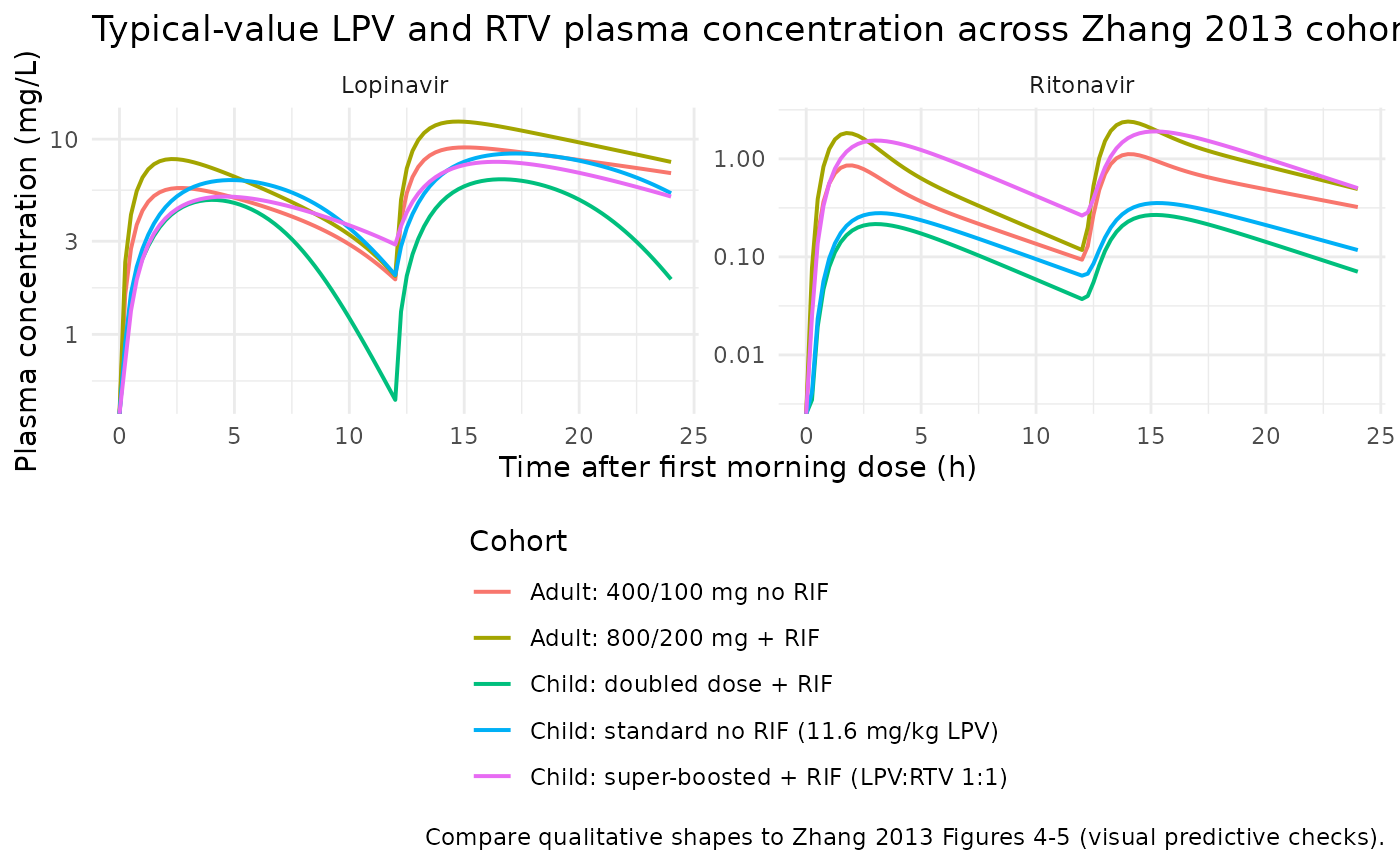
PKNCA validation – single dosing interval at steady state
Compute steady-state NCA over a single 12-hourly dosing interval. The cohort builder simulates 8 days at q12h dosing; the model reaches steady state well within 3 days for both LPV and RTV given their ~5 h half-lives. Lopinavir and ritonavir are computed separately because the source paper reports stratified Tmax and trough values per analyte.
# Steady-state NCA over the last complete morning-dose-to-evening-dose
# interval (the cohort builder uses n_days = 8L, so the last morning dose
# of the simulated horizon is at t = 84 h, and the immediately following
# evening dose at t = 96 h; we evaluate NCA over the interval [84, 96]).
start_ss <- 84
end_ss   <- 96

# LPV NCA
sim_lpv <- sim_typical |>
  dplyr::filter(!is.na(Cc), time >= start_ss - 0.5, time <= end_ss + 0.5) |>
  dplyr::transmute(id, time, Cc = Cc, treatment)

# Defensive time-zero anchor per (id, treatment): PKNCA needs a time-zero
# row to anchor AUC; for the steady-state interval we use the start of the
# interval as the local time-zero with the predicted concentration at that
# instant.
sim_lpv <- dplyr::bind_rows(
  sim_lpv,
  sim_lpv |> dplyr::distinct(id, treatment) |>
    dplyr::mutate(time = start_ss,
                  Cc   = NA_real_)
) |>
  dplyr::group_by(id, treatment) |>
  dplyr::arrange(time, .by_group = TRUE) |>
  tidyr::fill(Cc, .direction = "down") |>
  dplyr::ungroup() |>
  dplyr::distinct(id, treatment, time, .keep_all = TRUE)

dose_lpv <- events |>
  dplyr::filter(evid == 1L, cmt == "depot", time == 0) |>
  dplyr::transmute(id, time = start_ss, amt = amt, treatment)

conc_obj_lpv <- PKNCA::PKNCAconc(sim_lpv, Cc ~ time | treatment + id,
                                 concu = "mg/L", timeu = "h")
dose_obj_lpv <- PKNCA::PKNCAdose(dose_lpv, amt ~ time | treatment + id,
                                 doseu = "mg")

intervals_ss <- data.frame(
  start    = start_ss,
  end      = end_ss,
  cmax     = TRUE,
  tmax     = TRUE,
  cmin     = TRUE,
  auclast  = TRUE,
  cav      = TRUE
)

nca_lpv <- PKNCA::pk.nca(PKNCA::PKNCAdata(conc_obj_lpv, dose_obj_lpv,
                                          intervals = intervals_ss))

knitr::kable(
  as.data.frame(nca_lpv$result) |>
    dplyr::filter(PPTESTCD %in% c("cmax", "tmax", "cmin", "auclast")) |>
    dplyr::select(treatment, PPTESTCD, PPORRES) |>
    dplyr::mutate(PPORRES = signif(PPORRES, 4)) |>
    tidyr::pivot_wider(names_from = PPTESTCD, values_from = PPORRES),
  caption = paste("Lopinavir steady-state NCA over the [156, 168] h",
                  "interval (typical-value)."),
  align = c("l", "r", "r", "r", "r")
)| treatment | auclast | cmax | cmin | tmax |
|---|---|---|---|---|
| Adult: 400/100 mg no RIF | 125.90 | 12.040 | 5.2330 | 2.75 |
| Adult: 800/200 mg + RIF | 137.70 | 14.080 | 4.0580 | 2.50 |
| Child: doubled dose + RIF | 55.10 | 6.330 | 0.6203 | 4.50 |
| Child: standard no RIF (11.6 mg/kg LPV) | 95.98 | 9.503 | 3.5740 | 5.00 |
| Child: super-boosted + RIF (LPV:RTV 1:1) | 89.33 | 8.731 | 4.4070 | 4.00 |
sim_rtv <- sim_typical |>
  dplyr::filter(!is.na(Cc_rtv), time >= start_ss - 0.5, time <= end_ss + 0.5) |>
  dplyr::transmute(id, time, Cc = Cc_rtv, treatment)

sim_rtv <- dplyr::bind_rows(
  sim_rtv,
  sim_rtv |> dplyr::distinct(id, treatment) |>
    dplyr::mutate(time = start_ss, Cc = NA_real_)
) |>
  dplyr::group_by(id, treatment) |>
  dplyr::arrange(time, .by_group = TRUE) |>
  tidyr::fill(Cc, .direction = "down") |>
  dplyr::ungroup() |>
  dplyr::distinct(id, treatment, time, .keep_all = TRUE)

dose_rtv <- events |>
  dplyr::filter(evid == 1L, cmt == "depot_rtv", time == 0) |>
  dplyr::transmute(id, time = start_ss, amt = amt, treatment)

conc_obj_rtv <- PKNCA::PKNCAconc(sim_rtv, Cc ~ time | treatment + id,
                                 concu = "mg/L", timeu = "h")
dose_obj_rtv <- PKNCA::PKNCAdose(dose_rtv, amt ~ time | treatment + id,
                                 doseu = "mg")

nca_rtv <- PKNCA::pk.nca(PKNCA::PKNCAdata(conc_obj_rtv, dose_obj_rtv,
                                          intervals = intervals_ss))

knitr::kable(
  as.data.frame(nca_rtv$result) |>
    dplyr::filter(PPTESTCD %in% c("cmax", "tmax", "cmin", "auclast")) |>
    dplyr::select(treatment, PPTESTCD, PPORRES) |>
    dplyr::mutate(PPORRES = signif(PPORRES, 4)) |>
    tidyr::pivot_wider(names_from = PPTESTCD, values_from = PPORRES),
  caption = paste("Ritonavir steady-state NCA over the [156, 168] h",
                  "interval (typical-value)."),
  align = c("l", "r", "r", "r", "r")
)| treatment | auclast | cmax | cmin | tmax |
|---|---|---|---|---|
| Adult: 400/100 mg no RIF | 7.598 | 1.1450 | 0.12440 | 2.00 |
| Adult: 800/200 mg + RIF | 14.220 | 2.4250 | 0.14360 | 2.00 |
| Child: doubled dose + RIF | 1.986 | 0.2703 | 0.04140 | 3.25 |
| Child: standard no RIF (11.6 mg/kg LPV) | 2.834 | 0.3613 | 0.07537 | 3.25 |
| Child: super-boosted + RIF (LPV:RTV 1:1) | 14.120 | 1.9220 | 0.29440 | 3.25 |
Demonstrate the morning-vs-evening trough asymmetry
Zhang 2013 reports that the morning trough concentrations of lopinavir are higher than the evening trough concentrations in both adults and children, driven by (a) the +19% bioavailability boost at the evening LPV dose for adults and (b) the overnight (post-evening-dose) reduction in apparent clearance of both drugs in both populations (Results, paragraph “Diurnal variations”).
# At t = 11.75 h: evening trough = concentration immediately before the
# evening dose at t = 12 h (= post-morning-dose Ctrough).
# At t = 23.75 h: morning trough = concentration immediately before the
# next morning dose at t = 24 h (= post-evening-dose Ctrough).
sim_typical |>
  dplyr::filter(round(time, 2) %in% c(11.75, 23.75)) |>
  dplyr::transmute(treatment,
                   trough = ifelse(round(time, 2) == 11.75,
                                   "evening trough (post-AM)",
                                   "morning trough (post-PM)"),
                   Cc_lpv = round(Cc, 3),
                   Cc_rtv = round(Cc_rtv, 4)) |>
  knitr::kable(
    caption = paste("Typical-value LPV / RTV trough concentrations at the",
                    "12-h evening trough (post-morning dose) and the 24-h",
                    "morning trough (post-evening dose) on day 1."),
    align = c("l", "l", "r", "r")
)| treatment | trough | Cc_lpv | Cc_rtv |
|---|---|---|---|
| Adult: 400/100 mg no RIF | evening trough (post-AM) | 2.033 | 0.0981 |
| Adult: 400/100 mg no RIF | evening trough (post-AM) | 2.033 | 0.0981 |
| Adult: 400/100 mg no RIF | morning trough (post-PM) | 6.766 | 0.3307 |
| Adult: 400/100 mg no RIF | morning trough (post-PM) | 6.766 | 0.3307 |
| Adult: 800/200 mg + RIF | evening trough (post-AM) | 2.147 | 0.1245 |
| Adult: 800/200 mg + RIF | evening trough (post-AM) | 2.147 | 0.1245 |
| Adult: 800/200 mg + RIF | morning trough (post-PM) | 7.756 | 0.5091 |
| Adult: 800/200 mg + RIF | morning trough (post-PM) | 7.756 | 0.5091 |
| Child: standard no RIF (11.6 mg/kg LPV) | evening trough (post-AM) | 2.177 | 0.0675 |
| Child: standard no RIF (11.6 mg/kg LPV) | evening trough (post-AM) | 2.177 | 0.0675 |
| Child: standard no RIF (11.6 mg/kg LPV) | morning trough (post-PM) | 5.468 | 0.1217 |
| Child: standard no RIF (11.6 mg/kg LPV) | morning trough (post-PM) | 5.468 | 0.1217 |
| Child: super-boosted + RIF (LPV:RTV 1:1) | evening trough (post-AM) | 2.978 | 0.2797 |
| Child: super-boosted + RIF (LPV:RTV 1:1) | evening trough (post-AM) | 2.978 | 0.2797 |
| Child: super-boosted + RIF (LPV:RTV 1:1) | morning trough (post-PM) | 5.182 | 0.5246 |
| Child: super-boosted + RIF (LPV:RTV 1:1) | morning trough (post-PM) | 5.182 | 0.5246 |
| Child: doubled dose + RIF | evening trough (post-AM) | 0.523 | 0.0393 |
| Child: doubled dose + RIF | evening trough (post-AM) | 0.523 | 0.0393 |
| Child: doubled dose + RIF | morning trough (post-PM) | 2.075 | 0.0738 |
| Child: doubled dose + RIF | morning trough (post-PM) | 2.075 | 0.0738 |
The morning trough (concentration at 24 h, just before the next morning dose) is higher than the evening trough (concentration at 12 h, just before the evening dose) across the cohorts – consistent with Zhang 2013 Figure 3.
Assumptions and deviations
- Number of ritonavir transit compartments fixed at NN = 2. Zhang 2013 Table 2 does not list the number of transit compartments used for the ritonavir absorption chain. The adult-only precursor (Zhang et al. 2012, doi:10.1111/j.1365-2125.2011.04154.x, Table 2) reports NN = 2.03 (rounded to 2). The same paper develops the same structural absorption form carried forward to the combined adult+child Zhang 2013 model. We adopt NN = 2 fixed transit compartments here. Sensitivity to NN = 1 or NN = 3 was not investigated.
-
Ritonavir-dose effect on bioavailability is ADDITIVE in
absolute F units, not multiplicative. Zhang 2013 Methods
presents the paper formula
F = BIO + SLP * (DoseRTV - DoseRTV_STD). The Methods OCR is ambiguous about the+ vs *sign because the equation is rendered as a graphic in the source PDF, but the additive reading is the only one that reproduces Zhang 2013 Table 3 values exactly: super-boosted children (RTV 14 mg/kg, with RIF) -> LPV F = 0.33 + 0.019 * (14 - 2.9) = 0.541 (Table 3 = 0.53), RTV F = 0.021 + 0.026 * (14 - 2.9) = 0.310 (Table 3 = 0.31); doubled-dose children (RTV 6 mg/kg, with RIF) -> LPV F = 0.389 (Table 3 = 0.38), RTV F = 0.102 (Table 3 = 0.10). The multiplicative reading would give 0.400 / 0.027 / 0.349 / 0.023, all far from Table 3. The model implements the additive form. F can exceed 1 at very high ritonavir doses (e.g., adult RTV F = 1.21 at 3.08 mg/kg with RIF for an 80 kg adult on the 800/200 mg regimen); this reflects the paper’s linear-additive parameterisation and is not a numerical artifact. -
Diurnal effect indicator anchored to t = 0 = morning
dose. rxode2’s
tis the integration time. The model derivesevening_period = (t mod 24) >= 12and applies the overnight CL reduction continuously across that window and the evening-dose F boost at the dose event time. This implementation requires the simulation event table to alignt = 0to the morning dose. The Bienczak 2016 nevirapine model uses the samet mod 24pattern (continuous cosine wave on CL); seeinst/modeldb/specificDrugs/Bienczak_2016_nevirapine.Rlines 225-228. If a downstream user supplies an event table whose first dose is at t > 0 (e.g., a morning dose at t = 8 to align with clock-time 08:00), they must offset their dose times so that t = 0 corresponds to the morning dose, OR they should regard the diurnal terms in this model as not physiologically applicable to their use case. - Inter-occasion variability (IOV) NOT carried. Zhang 2013 Table 2 reports IOV on bioavailability (LPV 28%, RTV 43%), apparent CL (LPV 18%, RTV shared with LPV via a 100%-FIX correlation), absorption rate ka (LPV 68%), and MTT (RTV 39%). For a typical-value / population-IIV simulation use case, IOV is dropped here in favour of carrying only IIV; reproducing the paper’s per-occasion VPCs would require materialising per-subject random-effect deviations sampled per dosing occasion, which the packaged model does not enforce. A downstream user who needs the full source IOV structure can re-derive it from the per-occasion CV% values in Table 2.
- Within-drug IIV correlations NOT modelled. Zhang 2013 mentions “the correlations between the PK parameters both at IIV and IOV level were also investigated” but reports only the cross-drug correlation on IIV F (= 82%) and on IOV F (= 87%) in Table 2 ‘Correlation between lopinavir and ritonavir’ section. Within-drug correlations are treated as zero in the packaged model (e.g., the etalcl / etalvc within-LPV block is diagonal).
-
Additive residual error implemented on the lopinavir output
only. Zhang 2013 Table 2 reports a single additive-error value
(0.054 mg/L) whose row alignment with the column structure of the table
clusters it with the lopinavir-adult column. The ritonavir output uses
pure proportional error in the packaged model (21% CV per Table 2). If a
downstream user finds that the original paper intended a shared
additive-error term on both outputs, the model file’s
Cc_rtvresidual line can be amended; the impact on typical-value predictions is small relative to the proportional error magnitude.