Finerenone PK, UACR, serum potassium and eGFR (Snelder 2020)
Source:vignettes/articles/Snelder_2020_finerenone.Rmd
Snelder_2020_finerenone.RmdModel and source
- Citation: Snelder N, Heinig R, Drenth HJ, Joseph A, Kolkhof P, Lippert J, Garmann D, Ploeger B, Eissing T. Population Pharmacokinetic and Exposure-Response Analysis of Finerenone: Insights Based on Phase IIb Data and Simulations to Support Dose Selection for Pivotal Trials in Type 2 Diabetes with Chronic Kidney Disease. Clin Pharmacokinet. 2020;59(3):359-370.
- Article: https://doi.org/10.1007/s40262-019-00820-x
The paper contributes four models, all fitted to the pooled ARTS-DN and ARTS-DN Japan phase IIb data (the “final” ARTS-DN+JP models):
| Model | Endpoint | Source table |
|---|---|---|
Snelder_2020_finerenone |
finerenone plasma concentration | ESM Table S1 |
Snelder_2020_finerenone_uacr |
urinary albumin:creatinine ratio | ESM Table S2 |
Snelder_2020_finerenone_potassium |
serum potassium | ESM Table S3 |
Snelder_2020_finerenone_egfr |
eGFR (CKD-EPI) | ESM Table S4 |
The three PK/PD models were fitted sequentially, with individual post
hoc PK parameters from the final PK model as the input (ESM “Phase IIb
PK/PD Model Development”). Each PK/PD file therefore carries the PK
model with every PK parameter and PK variance wrapped in
fixed(); the PK residual error is not carried because
concentrations are not an output of those models.
mod_pk <- readModelDb("Snelder_2020_finerenone")
mod_uacr <- readModelDb("Snelder_2020_finerenone_uacr")
mod_k <- readModelDb("Snelder_2020_finerenone_potassium")
mod_egfr <- readModelDb("Snelder_2020_finerenone_egfr")
Population
ARTS-DN (NCT01874431, global, no sites in Japan) and ARTS-DN Japan (NCT01968668) randomised adults with type 2 diabetes and persistent albuminuria (UACR >= 30 mg/g) on a renin-angiotensin system blocker to placebo or finerenone 1.25, 2.5, 5, 7.5, 10, 15 or 20 mg once daily for 90 days. The PK/PD dataset held 893 subjects (799 ARTS-DN, 94 ARTS-DN Japan) and the PK dataset 787 subjects with 4597 quantifiable concentrations (paper Table 2). Median (5th-95th percentile) baseline body weight was 90.6 (64.1-126.3) kg in ARTS-DN and 71.6 (54-100) kg in ARTS-DN Japan; eGFR-MDRD was 63.9 (33.5-102.5) and 61.5 (41.0-87.2) mL/min/1.73 m^2; median age was 65 and 64 years (paper Table 3). The PK/PD dataset was 75.7% Caucasian, 9.1% non-Japanese Asian, 10.5% Japanese and 2.9% African American.
rxode2::rxode2(mod_pk)$population
#> ℹ parameter labels from comments will be replaced by 'label()'
#> $species
#> [1] "human"
#>
#> $n_subjects
#> [1] 787
#>
#> $n_studies
#> [1] 2
#>
#> $n_observations
#> [1] 4597
#>
#> $age_range
#> [1] "5th-95th percentile 49-78 years (ARTS-DN), 44-78 years (ARTS-DN Japan); medians 65 and 64 years"
#>
#> $weight_range
#> [1] "5th-95th percentile 64.1-126.3 kg (ARTS-DN, median 90.6), 54-100 kg (ARTS-DN Japan, median 71.6)"
#>
#> $egfr_mdrd_range
#> [1] "5th-95th percentile 33.5-102.5 mL/min/1.73 m^2 (ARTS-DN, median 63.9), 41.0-87.2 (ARTS-DN Japan, median 61.5)"
#>
#> $race_ethnicity
#>         Caucasian Asian_nonJapanese          Japanese  African_American
#>              75.7               9.1              10.5               2.9
#>             Other
#>               1.8
#>
#> $disease_state
#> [1] "type 2 diabetes with persistent albuminuria (UACR >= 30 mg/g) on a renin-angiotensin system blocker (diabetic kidney disease)"
#>
#> $dose_range
#> [1] "finerenone 1.25, 2.5, 5, 7.5, 10, 15 or 20 mg once daily orally for 90 days (plus placebo)"
#>
#> $regions
#> [1] "global (ARTS-DN, no sites in Japan) and Japan (ARTS-DN Japan)"
#>
#> $notes
#> [1] "PK dataset: 705 ARTS-DN plus 82 ARTS-DN Japan subjects with 4597 quantifiable observations (paper Table 2); 607 observations (11.3%) below the 0.1 ug/L LLOQ were excluded. Covariate percentiles are the PK/PD analysis dataset (paper Table 3; n = 893). Ethnicity percentages are the PK/PD dataset (paper Table 2). No ethnicity effect on PK was retained."
Source trace
| Quantity | Value | Source |
|---|---|---|
| Ka (depot and all three transits) | 10.7 1/h | ESM Table S1 (footnote d for the shared rate) |
| CL/F | 37.3 L/h | ESM Table S1 |
| Vc/F (= Vp/F) | 123 L | ESM Table S1; equal volumes per ESM “Phase IIa Models” and paper Discussion 4.1 |
| Q/F | 0.433 L/h | ESM Table S1 |
| Lag time | 0.215 h (fixed) | ESM Table S1 |
| F | 1 (fixed) | ESM Table S1 |
| BW slope on Vc/F | 0.449 | ESM Table S1 |
| eGFR-MDRD slope on CL/F and 1/F | 0.101 | ESM Table S1 |
| Covariate formulae and medians (88.5 kg, 63.53 mL/min/1.73 m^2) | - | ESM Table S1 footnotes |
| omega^2 Ka, CL/F, V/F, cov(CL/F, V/F) | 0.585, 0.2, 0.0927, 0.0928 | ESM Table S1 |
| PK proportional sigma^2 | 0.179 | ESM Table S1 |
| UACR baseline, screening UACR <= 300 / > 300 mg/g | 96.8 / 633 mg/g | ESM Table S2 (cat2 / cat3); paper Results 3.2.1 |
| UACR kout | 0.0014 1/h | ESM Table S2 |
| UACR Imax, IC50 | 1 (fixed), 12.9 ug/L | ESM Table S2; ESM Eq. S2 and S7 |
| UACR omega^2 baseline | 0.512 | ESM Table S2 |
| UACR additive sigma^2 (log scale); Japanese factor | 0.181; 0.692 | ESM Table S2 and footnote a |
| Potassium baseline; Japanese effect | 4.31 mmol/L; -3.13% | ESM Table S3 and footnote b |
| Potassium kin | 0.0815 mmol/L/h | ESM Table S3 |
| Potassium log-linear slope | 0.0204 | ESM Table S3 (footnote a); ESM Eq. S3 and S5 |
| Potassium omega^2 baseline (additive) | 0.102 | ESM Table S3 |
| Potassium proportional sigma^2; Japanese factor | 0.00432; 0.752 | ESM Table S3 and footnote c |
| eGFR-EPI baseline | 66.6 mL/min/1.73 m^2 | ESM Table S4 |
| eGFR kout | 0.0023 1/h | ESM Table S4 |
| eGFR power-model slope, exponent | 0.0359, 0.231 | ESM Table S4 (footnote a); ESM Eq. S2 and S6 |
| eGFR omega^2 baseline (additive); Japanese factor | 451; 0.647 | ESM Table S4 and footnote b |
| eGFR proportional sigma^2; Japanese factor | 0.00944; 0.675 | ESM Table S4 and footnote c |
Pharmacokinetics
Virtual cohorts
Body weight and eGFR-MDRD are drawn log-normally around the Table 3 medians, with log-scale SDs chosen so the 5th-95th percentiles approximately match Table 3. Covariates are drawn independently; their correlation is not reported.
set.seed(2020)
rxode2::rxSetSeed(2020)
n_arm <- 200

make_cohort <- function(n, wt_med, wt_p5, wt_p95, gfr_med, gfr_p5, gfr_p95,
                        japanese, id0) {
  data.frame(
    id = id0 + seq_len(n),
    WT = exp(rnorm(n, log(wt_med), log(wt_p95 / wt_p5) / (2 * 1.645))),
    CRCL = exp(rnorm(n, log(gfr_med), log(gfr_p95 / gfr_p5) / (2 * 1.645))),
    RACE_JAPANESE = japanese
  )
}

cohort_pk <- dplyr::bind_rows(
  make_cohort(n_arm, 90.6, 64.1, 126.3, 63.9, 33.5, 102.5, 0, 0) |>
    dplyr::mutate(study = "ARTS-DN"),
  make_cohort(n_arm, 71.6, 54, 100, 61.5, 41.0, 87.2, 1, 1000) |>
    dplyr::mutate(study = "ARTS-DN Japan")
)
Each subject receives finerenone 20 mg once daily for 30 days, with dense sampling over the last dosing interval (day 30, the Cmax,ss day of paper Figure 1).
dose_mg <- 20
obs_times <- 29 * 24 + seq(0, 24, by = 0.25)
ev_pk <- dplyr::bind_rows(
  cohort_pk |>
    dplyr::mutate(time = 0, evid = 1, amt = dose_mg, cmt = "depot", ii = 24, addl = 29),
  tidyr::crossing(cohort_pk, time = obs_times) |>
    dplyr::mutate(evid = 0, amt = 0, cmt = "central", ii = 0, addl = 0)
) |>
  dplyr::arrange(id, time, dplyr::desc(evid))

sim_pk <- rxode2::rxSolve(mod_pk, ev_pk, keep = "study", returnType = "data.frame")
#> ℹ parameter labels from comments will be replaced by 'label()'
sim_pk |>
  dplyr::mutate(tad = time - 29 * 24) |>
  dplyr::group_by(study, tad) |>
  dplyr::summarise(
    med = median(sim), lo = quantile(sim, 0.05), hi = quantile(sim, 0.95),
    .groups = "drop"
  ) |>
  ggplot(aes(tad, med)) +
  geom_ribbon(aes(ymin = lo, ymax = hi), fill = "grey80") +
  geom_line() +
  scale_y_log10() +
  facet_wrap(~study) +
  labs(x = "Time after dose (h)", y = "Finerenone (ug/L)")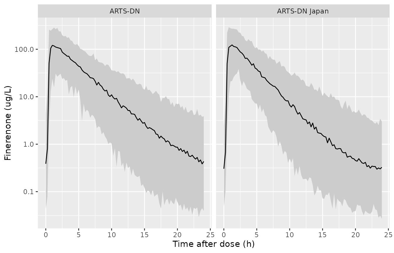
Simulated finerenone concentration over the day-30 dosing interval after 20 mg once daily (median and 90% prediction interval, including residual error). Compare with the ARTS-DN VPC of ESM Figure S1.
PKNCA: dose-normalised steady-state exposure
Paper Figure 1 reports the median dose-normalised AUCss (26.6 and 26.7 ug*h/L/mg) and Cmax,ss at day 30 (6.8 and 7.3 ug/L/mg) for ARTS-DN and ARTS-DN Japan, calculated from empirical Bayes estimates. The simulated concentrations are divided by the dose and analysed against a 1 mg dose.
conc_nca <- sim_pk |>
  dplyr::filter(!is.na(Cc)) |>
  dplyr::mutate(time = time - 29 * 24, Cdn = Cc / dose_mg) |>
  dplyr::select(id, study, time, Cdn)
dose_nca <- cohort_pk |>
  dplyr::distinct(id, study) |>
  dplyr::mutate(time = 0, amt = 1)

nca_res <- PKNCA::pk.nca(PKNCA::PKNCAdata(
  PKNCA::PKNCAconc(conc_nca, Cdn ~ time | study + id),
  PKNCA::PKNCAdose(dose_nca, amt ~ time | study + id),
  intervals = data.frame(start = 0, end = 24, auclast = TRUE, cmax = TRUE)
))

published_nca <- data.frame(
  study = c("ARTS-DN", "ARTS-DN Japan"),
  auclast = c(26.6, 26.7),
  cmax = c(6.8, 7.3)
)
cmp_nca <- nlmixr2lib::ncaComparisonTable(
  simulated = nca_res,
  reference = published_nca,
  by = "study",
  units = c(auclast = "ug*h/L per mg", cmax = "ug/L per mg"),
  tolerance_pct = 10
)
knitr::kable(cmp_nca, caption = "Median dose-normalised AUC0-24,ss and Cmax,ss: simulation versus paper Figure 1.")| NCA parameter | study | Reference | Simulated | % diff |
|---|---|---|---|---|
| Cmax (ug/L per mg) | ARTS-DN | 6.8 | 6.82 | +0.3% |
| Cmax (ug/L per mg) | ARTS-DN Japan | 7.3 | 7.18 | -1.6% |
| AUClast (ug*h/L per mg) | ARTS-DN | 26.6 | 28.5 | +7.2% |
| AUClast (ug*h/L per mg) | ARTS-DN Japan | 26.7 | 25.3 | -5.2% |
nca_med <- as.data.frame(nca_res$result) |>
  dplyr::filter(PPTESTCD %in% c("auclast", "cmax")) |>
  dplyr::group_by(study, PPTESTCD) |>
  dplyr::summarise(med = median(PPORRES), .groups = "drop") |>
  dplyr::left_join(
    tidyr::pivot_longer(published_nca, -study, names_to = "PPTESTCD", values_to = "ref"),
    by = c("study", "PPTESTCD")
  )
nca_med
#> # A tibble: 4 × 4
#>   study         PPTESTCD   med   ref
#>   <chr>         <chr>    <dbl> <dbl>
#> 1 ARTS-DN       auclast  28.5   26.6
#> 2 ARTS-DN       cmax      6.82   6.8
#> 3 ARTS-DN Japan auclast  25.3   26.7
#> 4 ARTS-DN Japan cmax      7.18   7.3
# Cohort medians: a mis-transcribed CL/F, volume or unit would move these by
# tens of percent.
stopifnot(all(abs(nca_med$med / nca_med$ref - 1) < 0.10))
Covariate effects on exposure
The paper states that a subject with eGFR-MDRD 30 mL/min/1.73 m^2 has a 32.9% higher AUCss and a 17.5% higher Cmax than a subject with eGFR-MDRD 90, and that a 50 kg subject has a 43.1% higher Cmax than a 100 kg subject (Results 3.1). These are typical-value contrasts. The eGFR contrast is reproduced exactly by the ARTS-DN-only slope (0.126, ESM Table S1, second column) and not by the final ARTS-DN+JP slope (0.101), so the quoted percentages were computed with the intermediate ARTS-DN-only model; both are shown. The ARTS-DN-only model differs from the final model in Ka, CL/F, Vc/F, Q/F and both covariate slopes (ESM Table S1); its covariate medians (90.4 kg, 63.9 mL/min/1.73 m^2) are not overridable here, so the final-model medians are used for both.
mod_pk_typ <- rxode2::zeroRe(mod_pk)
#> ℹ parameter labels from comments will be replaced by 'label()'
mod_pk_artsdn <- mod_pk_typ |>
  rxode2::ini(
    lka = log(11.4), lcl = log(36.9), lvc = log(125), lq = log(0.415),
    e_wt_vc = 0.516, e_crcl_cl = 0.126
  )
#> ℹ change initial estimate of `lka` to `2.43361335540045`
#> ℹ change initial estimate of `lcl` to `3.60821155104648`
#> ℹ change initial estimate of `lvc` to `4.8283137373023`
#> ℹ change initial estimate of `lq` to `-0.879476758751439`
#> ℹ change initial estimate of `e_wt_vc` to `0.516`
#> ℹ change initial estimate of `e_crcl_cl` to `0.126`

ss_metrics <- function(model, wt, crcl) {
  ev <- rxode2::et(amt = 1, ii = 24, addl = 29, cmt = "depot") |>
    rxode2::et(29 * 24 + seq(0, 24, by = 0.05), cmt = "central") |>
    as.data.frame() |>
    dplyr::mutate(WT = wt, CRCL = crcl)
  s <- as.data.frame(rxode2::rxSolve(model, ev))
  c(auc = sum(diff(s$time) * (head(s$Cc, -1) + tail(s$Cc, -1)) / 2), cmax = max(s$Cc))
}

contrast <- function(model) {
  g30 <- ss_metrics(model, 88.5, 30)
  g90 <- ss_metrics(model, 88.5, 90)
  w50 <- ss_metrics(model, 50, 63.53)
  w100 <- ss_metrics(model, 100, 63.53)
  100 * c(
    auc_egfr30_vs_90 = g30[["auc"]] / g90[["auc"]] - 1,
    cmax_egfr30_vs_90 = g30[["cmax"]] / g90[["cmax"]] - 1,
    cmax_wt50_vs_100 = w50[["cmax"]] / w100[["cmax"]] - 1
  )
}

tab_contrast <- data.frame(
  contrast = c("AUCss, eGFR 30 vs 90", "Cmax,ss, eGFR 30 vs 90", "Cmax,ss, BW 50 vs 100 kg"),
  paper = c(32.9, 17.5, 43.1),
  artsdn_only = contrast(mod_pk_artsdn),
  final = contrast(mod_pk_typ)
)
#> ℹ omega/sigma items treated as zero: 'etalka', 'etalcl', 'etalvc'
#> ℹ omega/sigma items treated as zero: 'etalka', 'etalcl', 'etalvc'
#> ℹ omega/sigma items treated as zero: 'etalka', 'etalcl', 'etalvc'
#> ℹ omega/sigma items treated as zero: 'etalka', 'etalcl', 'etalvc'
#> ℹ omega/sigma items treated as zero: 'etalka', 'etalcl', 'etalvc'
#> ℹ omega/sigma items treated as zero: 'etalka', 'etalcl', 'etalvc'
#> ℹ omega/sigma items treated as zero: 'etalka', 'etalcl', 'etalvc'
#> ℹ omega/sigma items treated as zero: 'etalka', 'etalcl', 'etalvc'
tab_contrast |>
  dplyr::rename(
    "Contrast (% higher)" = contrast,
    "Paper Results 3.1" = paper,
    "ARTS-DN-only parameters" = artsdn_only,
    "Final ARTS-DN+JP parameters" = final
  ) |>
knitr::kable(digits = 1, row.names = FALSE)| Contrast (% higher) | Paper Results 3.1 | ARTS-DN-only parameters | Final ARTS-DN+JP parameters |
|---|---|---|---|
| AUCss, eGFR 30 vs 90 | 32.9 | 32.9 | 25.4 |
| Cmax,ss, eGFR 30 vs 90 | 17.5 | 17.3 | 13.7 |
| Cmax,ss, BW 50 vs 100 kg | 43.1 | 42.6 | 35.0 |
# Closed-form typical-value contrasts: no random component, so a tight bound.
stopifnot(
  abs(tab_contrast$artsdn_only[1] - 32.9) < 0.3,
  abs(tab_contrast$artsdn_only[2] - 17.5) < 0.5,
  abs(tab_contrast$artsdn_only[3] - 43.1) < 3
)
The steady-state AUC for 1 mg is F / CL = 1 / 37.3 L/h = 26.8 ugh/L in the typical subject, matching the 26.6 ugh/L/mg median of Figure 1.
Pharmacodynamics
Typical time courses
typ_ev <- function(dose) {
  ev <- rxode2::et(seq(0, 180 * 24, by = 12), cmt = "central")
  if (dose > 0) ev <- rxode2::et(ev, amt = dose, ii = 24, addl = 179, cmt = "depot")
  as.data.frame(ev) |>
    dplyr::mutate(WT = 88.5, CRCL = 63.53, UACR = 200, RACE_JAPANESE = 0)
}
typ_run <- function(model, state, label) {
  dplyr::bind_rows(lapply(c(0, 10, 20), function(d) {
    s <- as.data.frame(rxode2::rxSolve(rxode2::zeroRe(model), typ_ev(d)))
    data.frame(time = s$time, value = s[[state]], dose = paste(d, "mg"), endpoint = label)
  }))
}
typ_pd <- dplyr::bind_rows(
  typ_run(mod_uacr, "uacr", "UACR (mg/g)"),
  typ_run(mod_k, "serum_k", "Serum potassium (mmol/L)"),
  typ_run(mod_egfr, "egfr", "eGFR-EPI (mL/min/1.73 m^2)")
)
#> ℹ parameter labels from comments will be replaced by 'label()'
#> Warning: No sigma parameters in the model
#> ℹ omega/sigma items treated as zero: 'etalka', 'etalcl', 'etalvc', 'etalrbase'
#> ℹ parameter labels from comments will be replaced by 'label()'
#> Warning: No sigma parameters in the model
#> ℹ omega/sigma items treated as zero: 'etalka', 'etalcl', 'etalvc', 'etalrbase'
#> ℹ parameter labels from comments will be replaced by 'label()'
#> Warning: No sigma parameters in the model
#> ℹ omega/sigma items treated as zero: 'etalka', 'etalcl', 'etalvc', 'etalrbase'
#> ℹ parameter labels from comments will be replaced by 'label()'
#> Warning: No sigma parameters in the model
#> ℹ omega/sigma items treated as zero: 'etalka', 'etalcl', 'etalvc', 'etarbase'
#> ℹ parameter labels from comments will be replaced by 'label()'
#> Warning: No sigma parameters in the model
#> ℹ omega/sigma items treated as zero: 'etalka', 'etalcl', 'etalvc', 'etarbase'
#> ℹ parameter labels from comments will be replaced by 'label()'
#> Warning: No sigma parameters in the model
#> ℹ omega/sigma items treated as zero: 'etalka', 'etalcl', 'etalvc', 'etarbase'
#> ℹ parameter labels from comments will be replaced by 'label()'
#> Warning: some etas defaulted to non-mu referenced, possible parsing error: etarbase
#> as a work-around try putting the mu-referenced expression on a simple line
#> Warning: No sigma parameters in the model
#> Warning: some etas defaulted to non-mu referenced, possible parsing error: etarbase
#> as a work-around try putting the mu-referenced expression on a simple line
#> ℹ omega/sigma items treated as zero: 'etalka', 'etalcl', 'etalvc', 'etarbase'
#> ℹ parameter labels from comments will be replaced by 'label()'
#> Warning: some etas defaulted to non-mu referenced, possible parsing error: etarbase
#> as a work-around try putting the mu-referenced expression on a simple line
#> Warning: No sigma parameters in the model
#> Warning: some etas defaulted to non-mu referenced, possible parsing error: etarbase
#> as a work-around try putting the mu-referenced expression on a simple line
#> ℹ omega/sigma items treated as zero: 'etalka', 'etalcl', 'etalvc', 'etarbase'
#> ℹ parameter labels from comments will be replaced by 'label()'
#> Warning: some etas defaulted to non-mu referenced, possible parsing error: etarbase
#> as a work-around try putting the mu-referenced expression on a simple line
#> Warning: No sigma parameters in the model
#> Warning: some etas defaulted to non-mu referenced, possible parsing error: etarbase
#> as a work-around try putting the mu-referenced expression on a simple line
#> ℹ omega/sigma items treated as zero: 'etalka', 'etalcl', 'etalvc', 'etarbase'
ggplot(typ_pd, aes(time / 24, value, colour = dose)) +
  geom_line() +
  facet_wrap(~endpoint, scales = "free_y") +
  labs(x = "Day", y = NULL, colour = "Dose")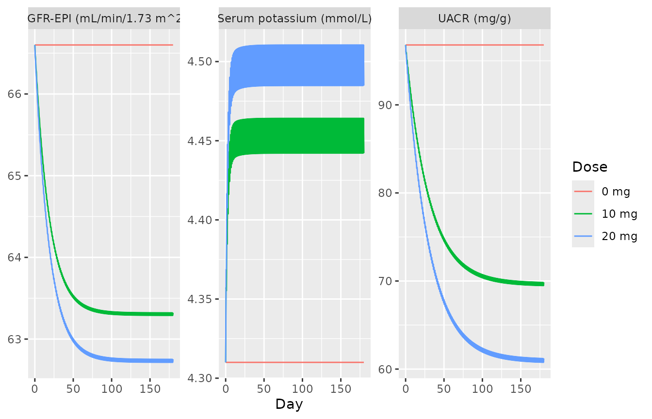
Typical-value response over 180 days of once-daily finerenone (median covariates, screening UACR <= 300 mg/g, non-Japanese).
Time to 99% of the steady-state drug effect
The abstract gives 138, 20 and 85 days for UACR, serum potassium and eGFR. The typical 20 mg response is evaluated once a day at trough, relative to its value after 400 days.
# A 400-day solve, so the last value is the steady state even for UACR
ev_t99 <- rxode2::et(amt = 20, ii = 24, addl = 399, cmt = "depot") |>
  rxode2::et(seq(0, 400 * 24, by = 24), cmt = "central") |>
  as.data.frame() |>
  dplyr::mutate(WT = 88.5, CRCL = 63.53, UACR = 200, RACE_JAPANESE = 0)
t99_days <- function(model, state) {
  s <- as.data.frame(rxode2::rxSolve(rxode2::zeroRe(model), ev_t99))
  frac <- (s[[state]] - s[[state]][1]) / (s[[state]][nrow(s)] - s[[state]][1])
  s$time[which(frac >= 0.99)[1]] / 24
}
t99 <- data.frame(
  endpoint = c("UACR", "Serum potassium", "eGFR-EPI"),
  days = c(t99_days(mod_uacr, "uacr"), t99_days(mod_k, "serum_k"), t99_days(mod_egfr, "egfr")),
  paper = c(138, 20, 85)
)
#> ℹ parameter labels from comments will be replaced by 'label()'
#> Warning: No sigma parameters in the model
#> ℹ omega/sigma items treated as zero: 'etalka', 'etalcl', 'etalvc', 'etalrbase'
#> ℹ parameter labels from comments will be replaced by 'label()'
#> Warning: No sigma parameters in the model
#> ℹ omega/sigma items treated as zero: 'etalka', 'etalcl', 'etalvc', 'etarbase'
#> ℹ parameter labels from comments will be replaced by 'label()'
#> Warning: some etas defaulted to non-mu referenced, possible parsing error: etarbase
#> as a work-around try putting the mu-referenced expression on a simple line
#> Warning: No sigma parameters in the model
#> Warning: some etas defaulted to non-mu referenced, possible parsing error: etarbase
#> as a work-around try putting the mu-referenced expression on a simple line
#> ℹ omega/sigma items treated as zero: 'etalka', 'etalcl', 'etalvc', 'etarbase'
knitr::kable(t99 |> dplyr::rename("Endpoint" = endpoint, "Simulated (days)" = days, "Paper (days)" = paper))| Endpoint | Simulated (days) | Paper (days) |
|---|---|---|
| UACR | 138 | 138 |
| Serum potassium | 20 | 20 |
| eGFR-EPI | 85 | 85 |
Scale of the baseline inter-individual variability
ESM Tables S3 and S4 print the baseline omega^2 for serum potassium (0.102) and eGFR-EPI (451) without stating the scale. Paper Table 3 gives the observed baseline percentiles, which include residual error. For eGFR a variance of 451 is only meaningful on the additive scale. For potassium the two readings differ enough for Table 3 to decide: an exponential IIV of variance 0.102 would put the 95th percentile of baseline potassium above 7 mmol/L. The quantiles below are computed from the model’s distributions (no ODE solve), so they are not subject to cohort sampling noise.
q <- c(0.05, 0.5, 0.95)
k_add <- qnorm(q, 4.31, sqrt(0.102 + 4.31^2 * 0.00432))
k_exp <- 4.31 * exp(qnorm(q, 0, sqrt(0.102 + 0.00432)))
g_add <- qnorm(q, 66.6, sqrt(451 + 66.6^2 * 0.00944))
tab_bl <- data.frame(
  quantity = rep(c("Serum potassium (mmol/L)", "eGFR-EPI (mL/min/1.73 m^2)"), each = 3),
  percentile = rep(c("5th", "50th", "95th"), 2),
  table3_artsdn = c(3.6, 4.3, 5.0, 33.3, 66.3, 101.3),
  additive_iiv = c(k_add, g_add),
  exponential_iiv = c(k_exp, rep(NA, 3))
)
tab_bl |>
  dplyr::rename(
    "Quantity" = quantity, "Percentile" = percentile,
    "Paper Table 3 (ARTS-DN)" = table3_artsdn,
    "Additive IIV (as coded)" = additive_iiv,
    "Exponential IIV (rejected)" = exponential_iiv
  ) |>
knitr::kable(digits = 2)| Quantity | Percentile | Paper Table 3 (ARTS-DN) | Additive IIV (as coded) | Exponential IIV (rejected) |
|---|---|---|---|---|
| Serum potassium (mmol/L) | 5th | 3.6 | 3.61 | 2.52 |
| Serum potassium (mmol/L) | 50th | 4.3 | 4.31 | 4.31 |
| Serum potassium (mmol/L) | 95th | 5.0 | 5.01 | 7.37 |
| eGFR-EPI (mL/min/1.73 m^2) | 5th | 33.3 | 30.08 | NA |
| eGFR-EPI (mL/min/1.73 m^2) | 50th | 66.3 | 66.60 | NA |
| eGFR-EPI (mL/min/1.73 m^2) | 95th | 101.3 | 103.12 | NA |
stopifnot(
  all(abs(k_add - c(3.6, 4.3, 5.0)) < 0.1),
  k_exp[3] > 7,
  # eGFR: the median and upper tail are compared tightly. The observed 5th
  # percentile is trimmed by the ARTS-DN eGFR >= 30 inclusion criterion,
  # which an untruncated normal IIV does not reproduce, so it may only sit
  # below the observed value, and by a few units.
  abs(g_add[2] - 66.3) < 1,
  abs(g_add[3] - 101.3) < 3,
  g_add[1] < 33.3,
  g_add[1] > 33.3 - 5
)
The approximation of the observed baseline as normal (IIV plus a proportional error evaluated at the typical baseline) is adequate here because both coefficients of variation are small. The simulated eGFR 5th percentile falls a few units below the observed one because ARTS-DN enrolled only patients with eGFR of at least 30 mL/min/1.73 m^2, which trims the lower tail of the observed baseline distribution.
Phase III dose-response scenario (paper Figure 3)
Paper Table 4 defines the scenario: 180 days of once-daily dosing with measurements on days 1, 30, 60, 90 and 180; eGFR 25-90 mL/min/1.73 m^2; serum potassium below 4.8 mmol/L at run-in and at screening. The cohort below uses the ARTS-DN body-weight and eGFR distributions with eGFR truncated to 25-90. The same event table drives all three PK/PD models.
Because UACR and eGFR are linear turnover models, the ratio of a subject’s response to its own baseline does not depend on the baseline. The percentage of subjects crossing a threshold is therefore computed from each simulated subject’s model-predicted ratio, with the residual error of the baseline and the follow-up measurement integrated analytically. This keeps Monte-Carlo noise from 200 subjects per arm out of percentages that are only a few percent.
cohort_ph3 <- function(n, id0) {
  crcl <- exp(rnorm(5 * n, log(63.9), log(102.5 / 33.5) / (2 * 1.645)))
  data.frame(
    id = id0 + seq_len(n),
    WT = exp(rnorm(n, log(90.6), log(126.3 / 64.1) / (2 * 1.645))),
    CRCL = head(crcl[crcl >= 25 & crcl <= 90], n),
    UACR = 200,
    RACE_JAPANESE = 0
  )
}
arms <- c(0, 10, 20, 30)
visit_days <- c(1, 30, 60, 90, 180)
ev_ph3 <- dplyr::bind_rows(lapply(seq_along(arms), function(i) {
  cov <- cohort_ph3(n_arm, 1000 * i) |> dplyr::mutate(arm = arms[i])
  obs <- tidyr::crossing(cov, time = (visit_days - 1) * 24) |>
    dplyr::mutate(evid = 0, amt = 0, ii = 0, addl = 0)
  if (arms[i] == 0) {
    return(obs)
  }
  dplyr::bind_rows(
    cov |> dplyr::mutate(time = 0, evid = 1, amt = arms[i], ii = 24, addl = 179, cmt = "depot"),
    obs
  )
})) |>
  dplyr::arrange(id, time, dplyr::desc(evid))

run_ph3 <- function(model, state) {
  ev <- ev_ph3 |> dplyr::mutate(cmt = ifelse(evid == 0, state, cmt))
  s <- rxode2::rxSolve(model, ev, keep = "arm", returnType = "data.frame")
  s |>
    dplyr::mutate(day = time / 24 + 1, value = .data[[state]]) |>
    dplyr::group_by(id) |>
    dplyr::mutate(ratio = value / value[day == 1]) |>
    dplyr::ungroup() |>
    dplyr::select(id, arm, day, ratio)
}
ph3_uacr <- run_ph3(mod_uacr, "uacr")
#> ℹ parameter labels from comments will be replaced by 'label()'
ph3_egfr <- run_ph3(mod_egfr, "egfr")
#> ℹ parameter labels from comments will be replaced by 'label()'
#> Warning: some etas defaulted to non-mu referenced, possible parsing error: etarbase
#> as a work-around try putting the mu-referenced expression on a simple line
ph3_k <- run_ph3(mod_k, "serum_k")
#> ℹ parameter labels from comments will be replaced by 'label()'
UACR targets
UACR is modelled on the log scale with residual SD
sqrt(0.181), so the log of an observed ratio has SD
sqrt(2 * 0.181) around the log of the predicted ratio.
sd_uacr <- sqrt(0.181)
targets <- c(0.8, 0.7, 0.6, 0.5)
pct_uacr <- ph3_uacr |>
  dplyr::filter(day == 180, arm > 0) |>
  dplyr::group_by(arm) |>
  dplyr::reframe(
    target = targets,
    pct = sapply(targets, function(x) 100 * mean(pnorm((log(x) - log(ratio)) / (sqrt(2) * sd_uacr))))
  )
ref_uacr <- data.frame(
  arm = rep(c(20, 30), each = 4),
  target = rep(targets, 2),
  paper = c(66.4, 58.6, 49.0, 39.5, 66.4 + 5.5, 58.6 + 5.2, 49.0 + 6.5, 39.5 + 5.7)
)
chk_uacr <- dplyr::inner_join(pct_uacr, ref_uacr, by = c("arm", "target"))
chk_uacr |>
  dplyr::mutate(target = paste("<=", target)) |>
  dplyr::rename(
    "Dose (mg QD)" = arm, "UACR day 180 / baseline" = target,
    "Simulated (%)" = pct, "Paper Results 3.3.1 (%)" = paper
  ) |>
knitr::kable(digits = 1)| Dose (mg QD) | UACR day 180 / baseline | Simulated (%) | Paper Results 3.3.1 (%) |
|---|---|---|---|
| 20 | <= 0.8 | 67.5 | 66.4 |
| 20 | <= 0.7 | 59.6 | 58.6 |
| 20 | <= 0.6 | 50.1 | 49.0 |
| 20 | <= 0.5 | 38.9 | 39.5 |
| 30 | <= 0.8 | 73.4 | 71.9 |
| 30 | <= 0.7 | 66.3 | 63.8 |
| 30 | <= 0.6 | 57.4 | 55.5 |
| 30 | <= 0.5 | 46.6 | 45.2 |
# Semi-analytic percentages over 200 PK-variable subjects: the centre and
# the envelope, not the extremes, are asserted.
stopifnot(
  abs(median(chk_uacr$pct - chk_uacr$paper)) < 4,
  max(abs(chk_uacr$pct - chk_uacr$paper)) < 6
)
ggplot(pct_uacr, aes(arm, pct, colour = factor(target))) +
  geom_line() +
  geom_point(data = ref_uacr, aes(y = paper), shape = 1, size = 3) +
  labs(x = "Finerenone dose (mg once daily)", y = "Subjects reaching target (%)", colour = "UACR ratio <=")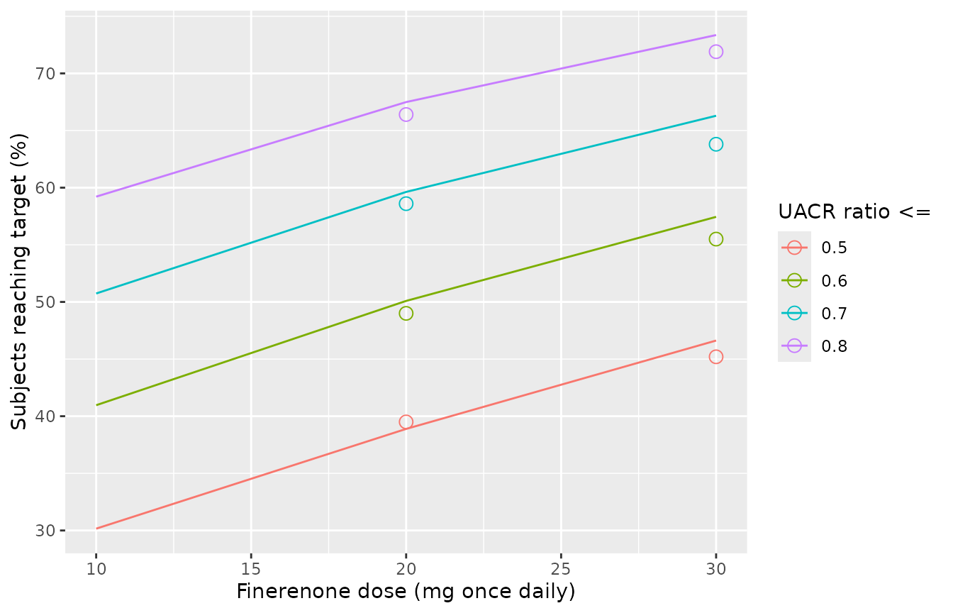
Percentage of subjects reaching each UACR target at day 180 by dose. Replicates Figure 3a of Snelder 2020 (points: values quoted in Results 3.3.1).
eGFR decreases
The eGFR residual error is proportional (SD
sqrt(0.00944)) on both the baseline and the day-180
measurement; the baseline error is integrated numerically.
sd_egfr <- sqrt(0.00944)
grid_e <- seq(-6, 6, length.out = 241)
w_e <- dnorm(grid_e) / sum(dnorm(grid_e))
p_drop <- function(r, x) {
  sum(w_e * pnorm(((1 - x) * (1 + sd_egfr * grid_e) / r - 1) / sd_egfr))
}
drops <- c(0.25, 0.30, 0.40)
pct_egfr <- ph3_egfr |>
  dplyr::filter(day == 180) |>
  dplyr::group_by(arm) |>
  dplyr::reframe(
    drop = drops,
    pct = sapply(drops, function(x) 100 * mean(sapply(ratio, p_drop, x = x)))
  )
ref_egfr <- data.frame(
  arm = c(20, 20, 30, 30),
  drop = c(0.25, 0.30, 0.25, 0.30),
  paper = c(5.0, 1.8, 5.5, 2.0)
)
chk_egfr <- dplyr::inner_join(pct_egfr, ref_egfr, by = c("arm", "drop"))
chk_egfr |>
  dplyr::mutate(drop = paste0(">= ", 100 * drop, "%")) |>
  dplyr::rename(
    "Dose (mg QD)" = arm, "eGFR decrease at day 180" = drop,
    "Simulated (%)" = pct, "Paper Results 3.3.3 (%)" = paper
  ) |>
knitr::kable(digits = 2)| Dose (mg QD) | eGFR decrease at day 180 | Simulated (%) | Paper Results 3.3.3 (%) |
|---|---|---|---|
| 20 | >= 25% | 5.06 | 5.0 |
| 20 | >= 30% | 1.70 | 1.8 |
| 30 | >= 25% | 5.60 | 5.5 |
| 30 | >= 30% | 1.92 | 2.0 |
stopifnot(
  all(abs(chk_egfr$pct - chk_egfr$paper) < 1),
  all(pct_egfr$pct[pct_egfr$drop == 0.40 & pct_egfr$arm %in% c(20, 30)] < 0.5)
)
The paper also states fewer than 0.1% of subjects lose 40% or more; the simulated values at 20 and 30 mg are 0.083 and 0.097%.
Serum potassium above 5.5 mmol/L
Unlike UACR and eGFR, this percentage depends on each subject’s baseline and on the screening rule, so the true baseline is integrated over its additive IIV distribution, N(4.31, 0.102). Inclusion requires the observed pre-treatment potassium to be below 4.8 mmol/L. Table 4 names two such measurements (run-in and screening); whether the day-1 measurement was also conditioned on is not stated, and the paper stresses that the result is highly sensitive to this rule (Discussion 4.3). Both readings are shown. The measurement ratios are taken from each subject’s own solve; after day 30 they are at steady state (20 days to 99%), where the ratio does not depend on the baseline.
sd_k <- sqrt(0.00432)
grid_k <- seq(-6, 6, length.out = 241)
w_k <- dnorm(grid_k) / sum(dnorm(grid_k))
r0 <- 4.31 + sqrt(0.102) * grid_k
p_exceed <- function(ratios, n_screen) {
  incl <- pnorm((4.8 / r0 - 1) / sd_k)^n_screen
  none <- sapply(r0, function(b) prod(pnorm((5.5 / (b * ratios) - 1) / sd_k)))
  sum(w_k * incl * (1 - none)) / sum(w_k * incl)
}
pct_k <- ph3_k |>
  dplyr::group_by(arm, id) |>
  dplyr::summarise(
    two = p_exceed(ratio, 2),
    three = p_exceed(ratio, 3),
    .groups = "drop"
  ) |>
  dplyr::group_by(arm) |>
  dplyr::summarise(two = 100 * mean(two), three = 100 * mean(three), .groups = "drop") |>
  dplyr::left_join(data.frame(arm = c(20, 30), paper = c(1.3, 1.7)), by = "arm")
pct_k |>
  dplyr::rename(
    "Dose (mg QD)" = arm,
    "Simulated, 2 screening values < 4.8 (%)" = two,
    "Simulated, 3 screening values < 4.8 (%)" = three,
    "Paper Results 3.3.2 (%)" = paper
  ) |>
knitr::kable(digits = 2)| Dose (mg QD) | Simulated, 2 screening values < 4.8 (%) | Simulated, 3 screening values < 4.8 (%) | Paper Results 3.3.2 (%) |
|---|---|---|---|
| 0 | 0.32 | 0.18 | NA |
| 10 | 1.10 | 0.71 | NA |
| 20 | 1.66 | 1.12 | 1.3 |
| 30 | 2.09 | 1.45 | 1.7 |
Assumptions and deviations
- Additive baseline IIV for serum potassium and eGFR. ESM Tables S3 and S4 print the baseline omega^2 without its scale, and the Methods state that random effects were exponential. The paper Table 3 baseline percentiles are reproduced only by an additive (normal) IIV for both endpoints (see “Scale of the baseline inter-individual variability”), so both are coded additively. The UACR baseline IIV is exponential, the natural scale for data the Methods say were log-transformed.
- “Ethnic effect on sigma^2” in ESM Table S4 is the baseline IIV. The footnote gives 291 for the Japanese population, which is 0.647 times the baseline omega^2 of 451; no global additive residual variance appears in the table. The factor is therefore applied to the baseline IIV variance.
-
Residual-variance factors for Japanese subjects
multiply variances, so the coded SDs are multiplied by the square root
of each factor.
RACE_JAPANESEis equivalent to the ARTS-DN Japan study indicator because ARTS-DN enrolled no Japanese subjects. -
UACR baseline categories. ESM Table S2 labels the
baselines “cat2” and “cat3”; the paper text defines the split as
screening UACR above 300 mg/g versus at or below it, which is how
UACRis used. -
Log-linear potassium effect. ESM Eq. S5 is read as
the natural logarithm,
log(Cc + 1)with Cc in ug/L. - Covariate time dependence. Whether body weight and eGFR-MDRD entered as baseline or time-varying values is not stated; the simulations use baseline values.
- PK in the PK/PD files. The PK/PD models were fitted to individual post hoc PK; the files instead carry the population PK model with its variability fixed, which reproduces the PK distribution rather than any individual.
- Covariate contrasts in Results 3.1 were evidently computed with the ARTS-DN-only PK model (ESM Table S1, second column): its eGFR slope reproduces 32.9% and 17.5% exactly, while the final slope gives the smaller values in the table above. The packaged model carries the final estimates.
- ESM Table S4 “ARTS-DN only” slope of 0.371 is ten times the final estimate (0.0359) and would suppress eGFR almost completely at clinical concentrations; it is presumably a misprint and is not used.
- Phase III threshold checks use typical PD parameters and no parameter uncertainty, whereas the paper simulated 5000 subjects per arm including NONMEM parameter uncertainty (ESM “Simulations”). Only the median percentages are compared.
-
rxode2 warns that
etarbasein the eGFR model is not mu-referenced because the Japanese factor scales the eta; the warning does not affect simulation.