Pyrazinamide (Jayanti 2026)
Source:vignettes/articles/Jayanti_2026_pyrazinamide.Rmd
Jayanti_2026_pyrazinamide.RmdModel and source
- Citation: Jayanti RP, Cho Y-S, Soedarsono S, Kim H-J, Kang J, Kim J, Oh JY, Kang BH, Ha JH, Kim J-W, Mertaniasih NM, Kusmiati T, Permatasari A, Yuliwulandari R, Kim R, Seong H-J, Ghim J-L, Kim D-H, Shin J-G; on behalf of the cPMTb. Population pharmacokinetics model of pyrazinamide to optimize tuberculosis treatment: An interethnic cohort study of diabetes mellitus effect on drug exposure. PLoS One. 2026;21(1):e0340133. doi:10.1371/journal.pone.0340133. Correction: PLoS One. 2026;21(4):e0347490. doi:10.1371/journal.pone.0347490 (corrects the funding statement only; no model parameter is affected).
- Description: One-compartment population pharmacokinetic model with first-order absorption and first-order elimination for oral pyrazinamide in Korean and Indonesian adults with drug-susceptible tuberculosis (Jayanti 2026); lean body weight is an allometric covariate on CL/F and Vd/F (fixed exponents 0.75 and 1), apparent clearance carries a separate typical value and a separate interindividual variance for each ethnicity, and diabetes mellitus raises CL/F by 23% in Indonesian patients and by 26% in Korean patients aged 60 years or older
- Article: https://doi.org/10.1371/journal.pone.0340133
- Correction (funding statement only): https://doi.org/10.1371/journal.pone.0347490
- Supporting information (S1-S4 Tables, S1-S5 Figs, and the deposited NONMEM dataset as S2 File): https://doi.org/10.1371/journal.pone.0340133#sec022
Jayanti 2026 is the interethnic successor to the same cPMTb group’s
Korean-only pyrazinamide (PZA) model, which this library also ships as
Kim_2023_pyrazinamide.
It pools 160 Korean and 160 Indonesian tuberculosis patients, matched
1:1 on body weight and age, to ask two questions: does ethnicity itself
change PZA disposition, and does diabetes mellitus (DM)?
The answers drive the unusual shape of the model. Ethnicity is not a covariate effect – “Ethnicity did not significantly affect the CL/F and Vd/F of PZA” – yet apparent clearance is nonetheless estimated separately per ethnicity, because the two countries’ diabetic patients differ in age: Indonesian diabetic patients tend to be under 60, Korean diabetic patients tend to be older. A single pooled diabetes term could not describe both, so the final model carries two clearance typical values, two clearance variances, and two different diabetes covariate forms, selected by ethnicity.
Population
The cPMTb cohort is a multinational prospective tuberculosis cohort spanning 22 hospitals in the Republic of Korea and one in Surabaya, Indonesia, recruiting between 2018-08-20 and 2021-11-03. Adults (>= 18 years) with drug-susceptible tuberculosis on a PZA-based regimen for at least two weeks were eligible; non-adherent, pregnant and multi-drug-resistant patients were excluded.
To remove demographic confounding from the interethnic comparison the authors matched patients between countries on body weight and age (maximum difference 5 kg and 5 years), using the smaller Indonesian sample as the reference. That gives the modelled cohort of 160 patients per ethnicity contributing 407 concentrations (240 Indonesian, 167 Korean – Indonesian inpatients generally contributed two samples each, Korean outpatients one).
Baseline characteristics (Table 1): median age 46 years (IQR 31-57), total body weight 55 kg (IQR 50-59.8), lean body weight 45.5 kg (IQR 40.8-49.3), height 165 cm (IQR 160-170), 38.4% female, median eGFR 105.5 mL/min/1.73 m^2. Seventy- seven patients (24.1%) had diabetes mellitus – 55 of 160 Indonesians against 22 of 160 Koreans – and 25 (7.8%) were both diabetic and aged 60 years or older.
Sampling was sparse and randomised: blood was drawn at a random time 0-24 h after the last dose. PZA was quantified by validated HPLC-ESI-MS/MS over 2.0-80.0 mg/L (LLOQ 2.0 mg/L). 117 below-LLOQ samples and 28 outlier patients were excluded; the authors report refitting the base model with the below-LLOQ records included and finding worse goodness-of-fit and poorer parameter precision.
The same information is available programmatically via the model’s
population metadata
(readModelDb("Jayanti_2026_pyrazinamide")()$population).
Source trace
Every ini() entry in
inst/modeldb/specificDrugs/Jayanti_2026_pyrazinamide.R
carries an in-file comment naming its origin. They are collected here
for review.
| Equation / parameter | Value | Source location |
|---|---|---|
| Structural model (1-cmt, first-order absorption and elimination) | n/a | Results, “Population pharmacokinetics model of PZA”; absorption-delay models all rejected |
lclIndonesian (CL/F, Indonesian) |
3.18 L/h | Table 2, CL/F Indonesian; = theta1 (RSE 4.7%) |
lclKorean (CL/F, Korean) |
3.5 L/h | Table 2, CL/F Korean; = theta2 (RSE 4.5%) |
lvc (Vd/F) |
52.8 L | Table 2, Vd/F (L) = theta5 (RSE 6.6%) |
lka (Ka) |
2.0 1/h | Table 2, Ka (h-1) = theta6 (RSE 15%) |
e_lbm_cl |
0.75 (fixed) | Methods, “fixed exponents of 0.75 for CL/F and 1 for Vd/F” |
e_lbm_vc |
1.0 (fixed) | Methods, same sentence |
| Lean-body-weight reference | 45 kg | Table 2 footnote d (see below) |
e_diab_cl (Indonesian DM) |
0.23 | Table 2, CL/F; DM = theta1 x (1 + theta3) (RSE
41.6%) |
e_age_ge60_diab_cl (Korean old DM) |
0.26 | Table 2, CL/F; Old DM = theta2 x (1 + theta4) (RSE
42.3%) |
| Retained covariate combination | DM in Indonesians, old DM in Koreans | Results, “we included DM (in Indonesians) - OldDM (in Koreans) as covariates of CL/F in the final model”; S1 Table row 1 |
| Geriatric-diabetes indicator | AGE_GE60 * DIS_DIAB |
Deposited dataset (S2 File) column OLDDM, which equals
OLD * DM exactly |
etalclIndonesian |
0.205 | Table 2, omega^2; CL/F Indonesian (%) = 20.5 |
etalclKorean |
0.05 | Table 2, omega^2; CL/F Korean (%) = 5 |
etalvc |
0.236 | Table 2, omega^2; Vd/F (%) = 23.6 |
| IIV on Ka | fixed to 0 (no eta) | Table 2, omega^2; Ka (%) = 0 (FIX)
|
addSd |
1.29 mg/L | Table 2, Residual variability / Additive (RSE
14.6%) |
The 45 kg allometric reference is only in the table image
The lean-body-weight value that every typical value in Table 2 refers to appears only in footnote d of Table 2:
Allometric scaling was applied to the CL/F and Vd/F data, and typical values reported here refer to the typical patient, with lean body weight of 45 kg.
That footnote is easy to lose. It survives in the publisher’s
rendered table image (pone.0340133.t002) and in a
layout-preserving text extraction of the PDF, but it is dropped entirely
by PDF-to-markdown conversion, which is the form most readers of this
article will work from. Without it the reference has to be inferred, and
the inference is ambiguous: back-solving the per-subgroup post-hoc CL/F
medians of S2 Table brackets it only to roughly 45-46 kg. The rounded
population median is 45.5 kg in Table 1 and 45.56 kg recomputed from the
deposited dataset, so 45 kg is the rounded median as the footnote
implies.
Reading the IIV scale
Table 2 labels its variability rows
omega^2; <parameter> (%), which on its own could mean
a variance, a CV%, or a variance expressed as a percentage. Three
independent lines of evidence agree that it is the variance
multiplied by 100, so that 20.5 means
omega^2 = 0.205:
-
Table 2’s own footnote a defines the symbol:
“
omega^2, variance of interindividual variability”. -
The same group uses the identical convention in Kim
2023, where it is pinned by a row printed as
3 (FIX)against the literal(0.03 FIX)of that paper’s deposited NONMEM control stream. -
It is the only reading compatible with this paper’s own
post-hoc spread. S2 Table gives the Korean non-old-DM CL/F
interquartile range as 3.22-3.91 L/h about a 3.47 L/h median. Removing
the lean-body-weight contribution leaves an empirical-Bayes log-scale
spread of about 0.093, which at the reported 56.9% shrinkage implies
omeganear 0.216 – against 0.224 predicted byomega^2 = 0.05, and 0.05 predicted by the CV% reading. The Indonesian arm points the same way.
# Line 3 above, evaluated. sd(eta_EBE) = omega * (1 - shrinkage), and the
# interquartile range of a normal spans 2 * qnorm(0.75) = 1.349 standard
# deviations.
iqr_to_sd <- function(q1, q3) log(q3 / q1) / (2 * qnorm(0.75))

# Korean, not old-DM: S2 Table CL/F IQR 3.22-3.91; Table 2 shrinkage 56.9%.
# The lean-body-weight term contributes 0.75 * sdlog(LBW) to the CL/F spread;
# Table 1 gives the Korean LBW IQR as 41.6-50.75 kg.
sd_ebe_kor  <- iqr_to_sd(3.22, 3.91)
sd_lbw_kor  <- 0.75 * iqr_to_sd(41.6, 50.75)
omega_kor   <- sqrt(max(sd_ebe_kor^2 - sd_lbw_kor^2, 0)) / (1 - 0.569)

tibble::tibble(
  Reading            = c("variance x 100 (used here)", "CV percent"),
  `Implied omega`    = c(sqrt(0.05), 0.05),
  `omega from S2 Table` = omega_kor
) |>
knitr::kable(digits = 3, caption = "Korean clearance: omega implied by each reading of Table 2, against omega recovered from the paper's own post-hoc interquartile range.")| Reading | Implied omega | omega from S2 Table |
|---|---|---|
| variance x 100 (used here) | 0.224 | 0.214 |
| CV percent | 0.050 | 0.214 |
# The CV% reading is not merely a worse fit, it is arithmetically impossible for
# the Indonesian arm: shrinkage can only make the post-hoc spread SMALLER than
# omega, yet the Indonesian non-DM post-hoc spread already exceeds the omega
# that reading would imply.
sd_ebe_ind <- iqr_to_sd(2.36, 3.8)   # S2 Table, Indonesian non-DM CL/F IQR
stopifnot(sd_ebe_ind > 0.205)        # > omega under the CV% reading (0.205)
stopifnot(sd_ebe_ind < sqrt(0.205))  # < omega under the variance reading (0.453)
Virtual cohort
Original observed data are not publicly available in a per-patient form suitable for re-simulation here, but the deposited NONMEM dataset (S2 File) is public and is used below only to check covariate coding, never as a parameter source.
The cohort mirrors the four subgroups Jayanti 2026 uses for its post-hoc exposure comparison in S2 Table and Fig 3: Indonesian with and without DM, and Korean split into “old DM” (>= 60 years old and diabetic) and “other patients”. Doses are 1,200 mg once daily, the normalising dose of S2 Table and Fig 3.
Lean body weight is drawn per ethnicity from a log-normal centred on the Table 1 medians (Korean 46.2 kg, Indonesian 44.9 kg) with a log-scale spread recovered from the Table 1 interquartile ranges, truncated to the range observed in the deposited dataset. The paper does not report lean body weight separately by diabetes stratum, so both strata of an ethnicity share a distribution.
rxode2::rxSetSeed(20260129)
set.seed(20260129)

dose_mg   <- 1200   # S2 Table and Fig 3 normalise exposures to 1,200 mg
tau       <- 24     # once daily
n_dose    <- 7      # 7 daily doses; t1/2 is about 10 h, so this is steady state
t_ss      <- tau * (n_dose - 1)
n_per_arm <- 200    # the per-arm cap

# Table 1 lean-body-weight medians and interquartile ranges, by ethnicity.
lbm_med <- c(Indonesian = 44.9,  Korean = 46.2)
lbm_sd  <- c(Indonesian = log(48.00 / 40.70) / (2 * qnorm(0.75)),
             Korean     = log(50.75 / 41.60) / (2 * qnorm(0.75)))
lbm_lo  <- 32.45    # deposited dataset (S2 File) observed range
lbm_hi  <- 68.17

# Observation grid: dense through the absorption phase (Tmax is near 1.6 h with
# Ka = 2.0 1/h) so the trapezoidal AUC does not understate the peak.
obs_grid <- sort(unique(c(seq(0, 4, by = 0.05), seq(4, tau, by = 0.25))))

make_arm <- function(n, arm, ethnicity, race_korean, dis_diab, age_ge60,
                     id_offset, sd_scale = 1) {
  subj <- tibble(
    id          = id_offset + seq_len(n),
    arm         = arm,
    RACE_KOREAN = race_korean,
    DIS_DIAB    = dis_diab,
    AGE_GE60    = age_ge60,
    LBM         = pmin(pmax(
      lbm_med[[ethnicity]] * exp(rnorm(n, 0, lbm_sd[[ethnicity]] * sd_scale)),
      lbm_lo), lbm_hi)
  )
  doses <- subj |>
    crossing(time = seq(0, tau * (n_dose - 1), by = tau)) |>
    mutate(amt = dose_mg, evid = 1L, cmt = "depot")
  obs <- subj |>
    crossing(time = t_ss + obs_grid) |>
    mutate(amt = NA_real_, evid = 0L, cmt = "central")
  bind_rows(doses, obs) |> arrange(id, time, desc(evid))
}

events <- bind_rows(
  make_arm(n_per_arm, "Indonesian, DM",     "Indonesian", 0, 1, 0, id_offset =   0L),
  make_arm(n_per_arm, "Indonesian, non-DM", "Indonesian", 0, 0, 0, id_offset = 200L),
  make_arm(n_per_arm, "Korean, old DM",     "Korean",     1, 1, 1, id_offset = 400L),
  make_arm(n_per_arm, "Korean, other",      "Korean",     1, 0, 0, id_offset = 600L)
)

# Disjoint IDs across arms are mandatory -- duplicate IDs silently merge.
stopifnot(!anyDuplicated(unique(events[, c("id", "time", "evid")])))

events |> count(arm, name = "rows")
#> # A tibble: 4 × 2
#>   arm                 rows
#>   <chr>              <int>
#> 1 Indonesian, DM     33600
#> 2 Indonesian, non-DM 33600
#> 3 Korean, old DM     33600
#> 4 Korean, other      33600
Typical-value check
A zeroRe()-style solve with every subject pinned at the
model’s 45 kg lean-body-weight reference must return Table 2’s thetas
exactly. These are deterministic quantities, so they are asserted at
machine tolerance rather than with a cohort-sized band.
mod <- readModelDb("Jayanti_2026_pyrazinamide")

typ_events <- bind_rows(
  make_arm(1, "Indonesian, DM",     "Indonesian", 0, 1, 0, id_offset = 1000L, sd_scale = 0),
  make_arm(1, "Indonesian, non-DM", "Indonesian", 0, 0, 0, id_offset = 1001L, sd_scale = 0),
  make_arm(1, "Korean, old DM",     "Korean",     1, 1, 1, id_offset = 1002L, sd_scale = 0),
  make_arm(1, "Korean, other",      "Korean",     1, 0, 0, id_offset = 1003L, sd_scale = 0),
  make_arm(1, "Korean, young DM",   "Korean",     1, 1, 0, id_offset = 1004L, sd_scale = 0)
) |>
  mutate(LBM = 45)   # pin at the Table 2 footnote d reference

sim_typ <- rxode2::rxSolve(
  mod, events = typ_events, omega = NA, sigma = NA,
  keep = c("arm", "LBM", "RACE_KOREAN", "DIS_DIAB", "AGE_GE60")
) |>
  as.data.frame() |>
  mutate(tad = time - t_ss)
#> Warning: some etas defaulted to non-mu referenced, possible parsing error: etalclKorean
#> as a work-around try putting the mu-referenced expression on a simple line

typ_par <- sim_typ |>
  group_by(arm) |>
  summarise(cl = first(cl), vc = first(vc), ka = first(ka), .groups = "drop")

# Table 2 arithmetic, written out independently of the model.
expected <- tibble::tribble(
  ~arm,                  ~cl_expected,
  "Indonesian, DM",      3.18 * (1 + 0.23),
  "Indonesian, non-DM",  3.18,
  "Korean, old DM",      3.50 * (1 + 0.26),
  "Korean, other",       3.50,
  "Korean, young DM",    3.50   # DM alone is NOT a Korean covariate
)

chk_typ <- typ_par |> left_join(expected, by = "arm")
stopifnot(
  nrow(chk_typ) == 5L,
  !anyNA(chk_typ$cl_expected),
  max(abs(chk_typ$cl - chk_typ$cl_expected)) < 1e-8,
  max(abs(chk_typ$vc - 52.8)) < 1e-8,
  max(abs(chk_typ$ka - 2.0)) < 1e-8
)

chk_typ |>
  rename("Subgroup" = arm, "CL/F (L/h)" = cl, "Vd/F (L)" = vc,
         "Ka (1/h)" = ka, "CL/F expected from Table 2 (L/h)" = cl_expected) |>
knitr::kable(digits = 4, caption = "Typical-value parameters at the 45 kg lean-body-weight reference of Table 2 footnote d. Table 2 gives CL/F = 3.18 (Indonesian) and 3.5 (Korean) L/h, Vd/F = 52.8 L and Ka = 2.0 1/h; the Results text quotes 3.88 and 4.38 L/h for Indonesian and older Korean diabetic patients, against 3.91 and 4.41 here (the table's values are rounded to two significant figures).")| Subgroup | CL/F (L/h) | Vd/F (L) | Ka (1/h) | CL/F expected from Table 2 (L/h) |
|---|---|---|---|---|
| Indonesian, DM | 3.9114 | 52.8 | 2 | 3.9114 |
| Indonesian, non-DM | 3.1800 | 52.8 | 2 | 3.1800 |
| Korean, old DM | 4.4100 | 52.8 | 2 | 4.4100 |
| Korean, other | 3.5000 | 52.8 | 2 | 3.5000 |
| Korean, young DM | 3.5000 | 52.8 | 2 | 3.5000 |
Note the fifth row. A Korean diabetic patient younger than 60 takes the Korean reference clearance unmodified, because diabetes enters the Korean arm only crossed with age; this is exactly what the Results mean by “3.5 L/h for younger Korean patients with DM”. An Indonesian diabetic patient takes the 23% increase at any age.
Steady-state mass balance
At steady state under linear one-compartment kinetics, AUC over one
dosing interval equals Dose / (CL/F) exactly, whatever the
absorption model. Both sides use the same drawn parameters, so the only
difference is trapezoidal error and the bound can be tight.
mb <- sim_typ |>
  filter(!is.na(Cc), tad >= 0) |>
  group_by(arm) |>
  summarise(
    auc_trapz = sum(diff(tad) * (head(Cc, -1) + tail(Cc, -1)) / 2),
    auc_ident = dose_mg / first(cl),
    .groups   = "drop"
  ) |>
  mutate(pct_diff = 100 * (auc_trapz - auc_ident) / auc_ident)

# Deterministic: both sides use the same drawn parameters, so the only error is
# trapezoidal. Realised max 0.005% on the grid above; 0.1% still goes red if the
# observation grid is ever coarsened enough to understate the peak.
stopifnot(nrow(mb) == 5L, max(abs(mb$pct_diff)) < 0.1)

mb |>
  rename("Subgroup" = arm, "AUC0-24 (trapezoid, mg*h/L)" = auc_trapz,
         "Dose / (CL/F) (mg*h/L)" = auc_ident, "Difference (%)" = pct_diff) |>
knitr::kable(digits = c(0, 2, 2, 4), caption = "Steady-state AUC0-24 equals Dose/(CL/F) for the typical subject in every subgroup.")| Subgroup | AUC0-24 (trapezoid, mg*h/L) | Dose / (CL/F) (mg*h/L) | Difference (%) |
|---|---|---|---|
| Indonesian, DM | 306.79 | 306.80 | -0.0016 |
| Indonesian, non-DM | 377.34 | 377.36 | -0.0053 |
| Korean, old DM | 272.11 | 272.11 | -0.0012 |
| Korean, other | 342.85 | 342.86 | -0.0027 |
| Korean, young DM | 342.85 | 342.86 | -0.0027 |
This identity also holds in the paper’s own numbers, which is worth
recording because it does not hold in the predecessor
Kim 2023 (whose published AUC0-24 column is about half of
Dose/(CL/F)). Every one of the six S2 Table subgroups here
reconciles to within 1.5%:
s2 <- tibble::tribble(
  ~group,                ~cl_pub, ~auc_pub,
  "Korean, old DM",         4.61,    261.4,
  "Korean, other",          3.47,    345.7,
  "Korean, total",          3.52,    343.2,
  "Indonesian, DM",         3.74,    322.2,
  "Indonesian, non-DM",     3.12,    388.6,
  "Indonesian, total",      3.23,    371.1
) |>
  mutate(auc_from_cl = 1200 / cl_pub,
         pct_diff    = 100 * (auc_pub - auc_from_cl) / auc_from_cl)

# Deterministic -- both columns are transcribed published constants. Realised
# max 1.04%, consistent with the tables' 3-4 significant figures.
stopifnot(max(abs(s2$pct_diff)) < 1.5)

s2 |>
  rename("S2 Table subgroup" = group, "Published CL/F (L/h)" = cl_pub,
         "Published AUC0-24 (mg*h/L)" = auc_pub,
         "1200 / CL/F (mg*h/L)" = auc_from_cl, "Difference (%)" = pct_diff) |>
knitr::kable(digits = c(0, 2, 1, 1, 2), caption = "The published S2 Table is internally consistent: its AUC0-24 column reproduces Dose/(CL/F) from its own CL/F column.")| S2 Table subgroup | Published CL/F (L/h) | Published AUC0-24 (mg*h/L) | 1200 / CL/F (mg*h/L) | Difference (%) |
|---|---|---|---|---|
| Korean, old DM | 4.61 | 261.4 | 260.3 | 0.42 |
| Korean, other | 3.47 | 345.7 | 345.8 | -0.04 |
| Korean, total | 3.52 | 343.2 | 340.9 | 0.67 |
| Indonesian, DM | 3.74 | 322.2 | 320.9 | 0.42 |
| Indonesian, non-DM | 3.12 | 388.6 | 384.6 | 1.04 |
| Indonesian, total | 3.23 | 371.1 | 371.5 | -0.11 |
Replicate published figures
# Analogous to Fig 2 of Jayanti 2026 (prediction-corrected VPC): the spread of
# PZA concentrations across one steady-state dosing interval. The paper plots
# the observed median inside a 90% prediction interval.
sim |>
  filter(!is.na(Cc)) |>
  group_by(arm, tad) |>
  summarise(Q05 = quantile(Cc, 0.05), Q50 = quantile(Cc, 0.50),
            Q95 = quantile(Cc, 0.95), .groups = "drop") |>
  ggplot(aes(tad, Q50)) +
  geom_ribbon(aes(ymin = Q05, ymax = Q95), alpha = 0.25, fill = "steelblue") +
  geom_line(colour = "steelblue", linewidth = 0.8) +
  facet_wrap(~arm) +
  labs(x = "Time after dose (h)", y = "PZA concentration (mg/L)",
       title = "Steady-state PZA concentrations, 1,200 mg once daily",
       caption = paste("Median with 5th-95th percentile band,", n_per_arm,
                       "simulated subjects per arm. Analogous to Fig 2 of Jayanti 2026."))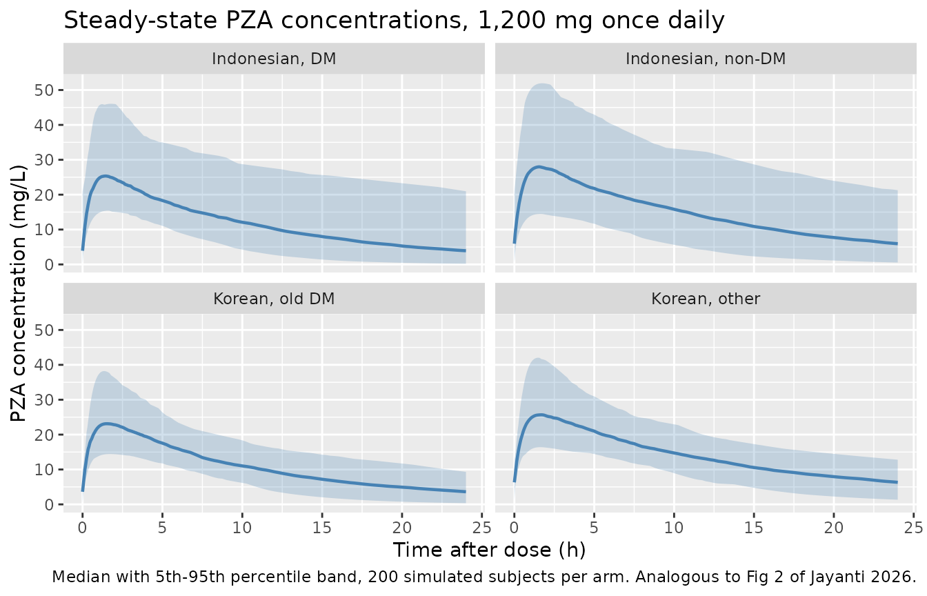
# Replicates Fig 3 of Jayanti 2026: AUC0-24, Cmax and CL/F contrasted between
# the DM and non-DM strata of each ethnicity.
per_subject <- sim |>
  filter(!is.na(Cc), tad >= 0) |>
  group_by(arm, id) |>
  summarise(
    Cmax   = max(Cc),
    `CL/F` = first(cl),
    `Vd/F` = first(vc),
    AUC024 = sum(diff(tad) * (head(Cc, -1) + tail(Cc, -1)) / 2),
    .groups = "drop"
  )

per_subject |>
  pivot_longer(c(AUC024, Cmax, `CL/F`), names_to = "metric", values_to = "value") |>
  mutate(metric = recode(metric,
    AUC024 = "AUC0-24 (mg*h/L)", Cmax = "Cmax (mg/L)", `CL/F` = "CL/F (L/h)")) |>
  ggplot(aes(arm, value, fill = arm)) +
  geom_boxplot(outlier.size = 0.4, show.legend = FALSE) +
  facet_wrap(~metric, scales = "free_y") +
  labs(x = NULL, y = NULL,
       title = "Exposure and clearance by ethnicity and diabetes stratum (1,200 mg daily)",
       caption = "Replicates Fig 3 of Jayanti 2026.") +
  theme(axis.text.x = element_text(angle = 30, hjust = 1))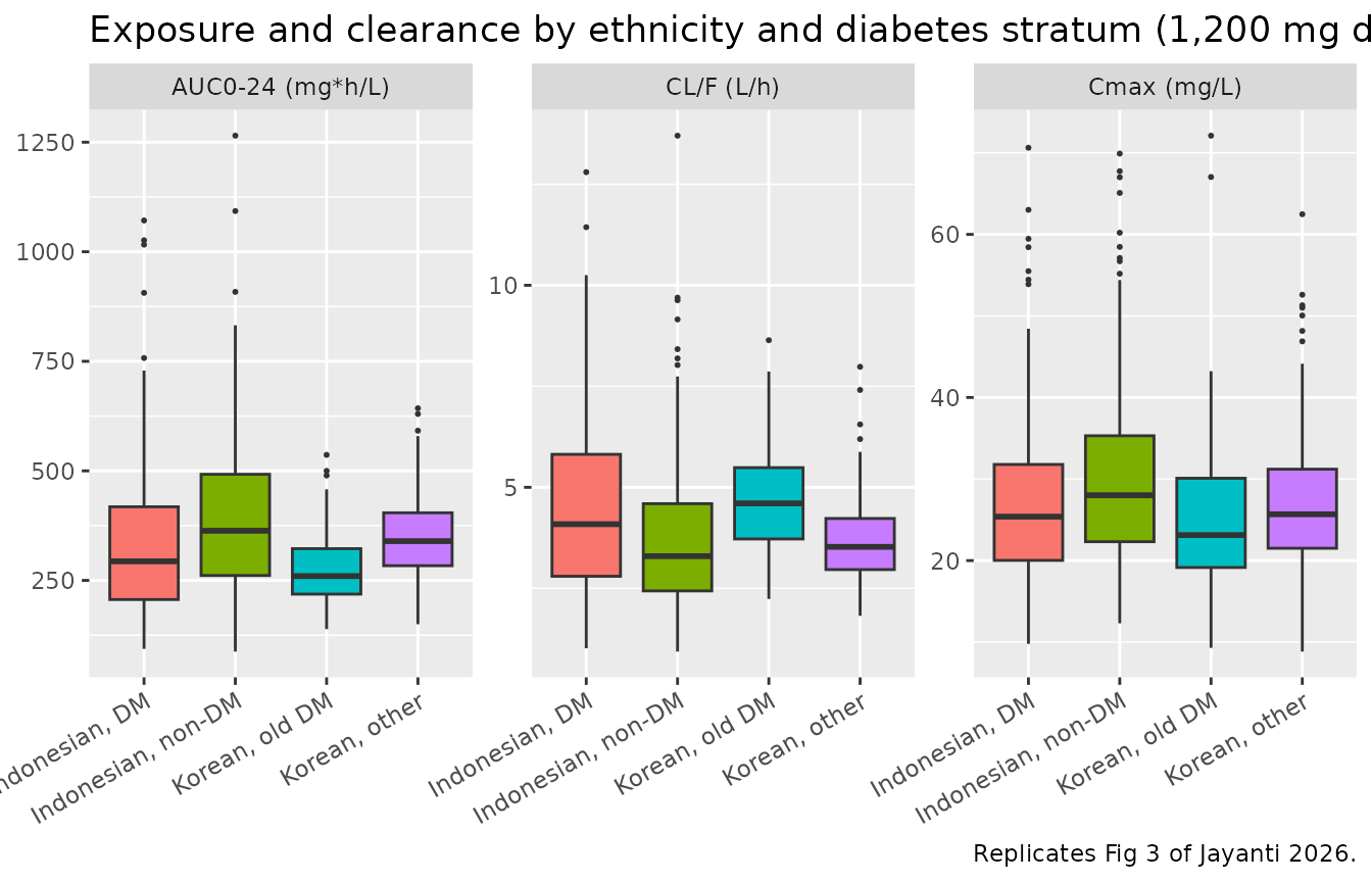
The model reproduces the paper’s qualitative ordering: within each ethnicity the diabetic stratum has the higher CL/F and the lower exposure, and the Korean old-DM arm has the lowest exposure of the four – “Compared to Indonesian TB-DM patients, older DM patients among Korean subjects had the lowest exposure of PZA”.
PKNCA validation
Steady-state NCA over the final dosing interval. The NCA runs on
Cc, the individual prediction, rather than on
sim: S2 Table’s values are post-hoc model-derived
quantities with no residual error in them, and Cmax taken
from a residual-error-carrying simulation is biased upward.
sim_nca <- sim |>
  filter(!is.na(Cc)) |>
  select(id, time, Cc, arm)

conc_obj <- PKNCA::PKNCAconc(sim_nca, Cc ~ time | arm + id,
                             concu = "mg/L", timeu = "h")

dose_df <- events |>
  filter(evid == 1) |>
  select(id, time, amt, arm)

dose_obj <- PKNCA::PKNCAdose(dose_df, amt ~ time | arm + id,
                             route = "extravascular", doseu = "mg")

intervals <- data.frame(
  start = t_ss, end = t_ss + tau,
  cmax = TRUE, tmax = TRUE, cmin = TRUE, auclast = TRUE, cav = TRUE
)

nca_res <- PKNCA::pk.nca(PKNCA::PKNCAdata(conc_obj, dose_obj, intervals = intervals))
as.data.frame(nca_res) |>
  filter(PPTESTCD %in% c("cmax", "tmax", "cmin", "auclast", "cav")) |>
  group_by(arm, PPTESTCD) |>
  summarise(median = median(PPORRES), .groups = "drop") |>
  pivot_wider(names_from = PPTESTCD, values_from = median) |>
  rename("Subgroup" = arm, "AUC0-24 (mg*h/L)" = auclast, "Cavg (mg/L)" = cav,
         "Cmax (mg/L)" = cmax, "Cmin (mg/L)" = cmin, "Tmax (h)" = tmax) |>
knitr::kable(digits = 2, caption = paste0("Simulated steady-state NCA (medians of ", n_per_arm, " subjects per arm), 1,200 mg once daily."))| Subgroup | AUC0-24 (mg*h/L) | Cavg (mg/L) | Cmax (mg/L) | Cmin (mg/L) | Tmax (h) |
|---|---|---|---|---|---|
| Indonesian, DM | 324.91 | 13.54 | 25.60 | 5.60 | 1.65 |
| Indonesian, non-DM | 391.11 | 16.30 | 30.26 | 6.57 | 1.65 |
| Korean, old DM | 264.55 | 11.02 | 22.82 | 3.51 | 1.60 |
| Korean, other | 337.29 | 14.05 | 27.05 | 5.86 | 1.65 |
Comparison against published NCA
S2 Table reports median post-hoc Cmax and AUC0-24, normalised to 1,200 mg, for exactly these four subgroups.
published <- tibble::tribble(
  ~arm,                  ~cmax,  ~auclast,
  "Indonesian, DM",       25.27,    322.2,
  "Indonesian, non-DM",   28.70,    388.6,
  "Korean, old DM",       21.46,    261.4,
  "Korean, other",        25.83,    345.7
)

cmp <- nlmixr2lib::ncaComparisonTable(
  simulated     = nca_res,
  reference     = published,
  by            = "arm",
  params        = c("cmax", "auclast"),
  units         = c(cmax = "mg/L", auclast = "mg*h/L"),
  tolerance_pct = 20
)

knitr::kable(cmp,
  caption = "Simulated vs. published (S2 Table) steady-state NCA at 1,200 mg once daily. * differs from reference by >20%.",
align = c("l", "l", "r", "r", "r"))| NCA parameter | arm | Reference | Simulated | % diff |
|---|---|---|---|---|
| Cmax (mg/L) | Indonesian, DM | 25.3 | 25.6 | +1.3% |
| Cmax (mg/L) | Indonesian, non-DM | 28.7 | 30.3 | +5.4% |
| Cmax (mg/L) | Korean, old DM | 21.5 | 22.8 | +6.4% |
| Cmax (mg/L) | Korean, other | 25.8 | 27 | +4.7% |
| AUClast (mg*h/L) | Indonesian, DM | 322 | 325 | +0.8% |
| AUClast (mg*h/L) | Indonesian, non-DM | 389 | 391 | +0.6% |
| AUClast (mg*h/L) | Korean, old DM | 261 | 265 | +1.2% |
| AUClast (mg*h/L) | Korean, other | 346 | 337 | -2.4% |
# Cohort-derived quantities, so the bound is on the CENTRE and is set with
# headroom over the sampling noise, not tightened to one run. With 200 subjects
# per arm the median of a log-normal with the Indonesian omega of 0.45 carries a
# standard error near 4%, and the systematic subgroup differences below run
# 2-8%. A 20% bound still goes red on a mis-transcribed clearance, dose, volume
# or unit, each of which moves these numbers by tens of percent.
sim_med <- as.data.frame(nca_res) |>
  filter(PPTESTCD %in% c("cmax", "auclast")) |>
  group_by(arm, PPTESTCD) |>
  summarise(sim = median(PPORRES), .groups = "drop") |>
  pivot_wider(names_from = PPTESTCD, values_from = sim)

gate <- published |>
  rename(cmax_pub = cmax, auclast_pub = auclast) |>
  left_join(sim_med, by = "arm") |>
  mutate(cmax_pct = 100 * (cmax - cmax_pub) / cmax_pub,
         auc_pct  = 100 * (auclast - auclast_pub) / auclast_pub)

stopifnot(
  nrow(gate) == 4L,                      # guard against a silent zero-row join
  !anyNA(gate$cmax), !anyNA(gate$auclast),
  max(abs(gate$cmax_pct)) < 20,
  max(abs(gate$auc_pct))  < 20
)

gate |>
  select(arm, cmax_pct, auc_pct) |>
  rename("Subgroup" = arm, "Cmax difference (%)" = cmax_pct,
         "AUC0-24 difference (%)" = auc_pct) |>
knitr::kable(digits = 1, caption = "Simulated minus published, as a percentage of published.")| Subgroup | Cmax difference (%) | AUC0-24 difference (%) |
|---|---|---|
| Indonesian, DM | 1.3 | 0.8 |
| Indonesian, non-DM | 5.4 | 0.6 |
| Korean, old DM | 6.4 | 1.2 |
| Korean, other | 4.7 | -2.4 |
Apparent volume of distribution agrees too, though with visibly more
scatter than clearance – unsurprisingly, since Vd/F carries
the model’s largest variance (omega^2 = 0.236) and is the
parameter that randomly-timed single samples identify worst (24.6%
shrinkage).
vd_pub <- c("Indonesian, DM" = 51.27, "Indonesian, non-DM" = 48.29,
            "Korean, old DM" = 56.72, "Korean, other" = 50.60)

vd_cmp <- per_subject |>
  group_by(arm) |>
  summarise(vd_sim = median(`Vd/F`), .groups = "drop") |>
  mutate(vd_pub = vd_pub[arm],
         pct    = 100 * (vd_sim - vd_pub) / vd_pub)

# Cohort-derived, and noisier than the clearance-driven metrics: the median of
# 200 draws from a log-normal with total log-scale spread near 0.51 has a
# standard error of about 4.5%, so the realised -3 to +9% scatter is sampling
# noise about a correct centre rather than bias. 25% retains headroom over that
# while still going red on a mis-transcribed volume or allometric exponent.
stopifnot(nrow(vd_cmp) == 4L, !anyNA(vd_cmp$vd_pub), max(abs(vd_cmp$pct)) < 25)

vd_cmp |>
  rename("Subgroup" = arm, "Simulated Vd/F (L)" = vd_sim,
         "S2 Table Vd/F (L)" = vd_pub, "Difference (%)" = pct) |>
knitr::kable(digits = 1, caption = "Apparent volume of distribution, simulated median against S2 Table.")| Subgroup | Simulated Vd/F (L) | S2 Table Vd/F (L) | Difference (%) |
|---|---|---|---|
| Indonesian, DM | 54.5 | 51.3 | 6.3 |
| Indonesian, non-DM | 46.4 | 48.3 | -3.9 |
| Korean, old DM | 52.9 | 56.7 | -6.7 |
| Korean, other | 53.1 | 50.6 | 4.9 |
Probability of target attainment
Jayanti 2026’s dose recommendations rest on the probability of
attaining AUC0-24 >= 363 mg*h/L. Because steady-state
AUC0-24 is exactly Dose/(CL/F) – the identity
gated above – the attainment probability can be read straight off the
model’s own simulated clearances without a second ODE solve.
Lean body weight per WHO weight band is taken from the deposited
dataset (S2 File) rather than reconstructed from the paper’s
virtual-population body weights, because the Boer equation the paper
uses to derive lean body weight extrapolates badly at low body weight:
applied to the paper’s own <40 kg virtual population
(34.75 kg) at the cohort median height it returns a lean body weight of
about 39 kg, i.e. greater than total body weight. That
pathology is real in the deposited data too – 12 of its 300 patients
have a lean body weight exceeding their total body weight.
bands <- tibble::tribble(
  ~band,       ~lbm_med, ~lbm_sdlog,
  "<40 kg",       36.84,     0.0644,
  "40-54 kg",     42.34,     0.1030,
  "55-70 kg",     49.26,     0.0734,
  ">70 kg",       57.10,     0.0299
)

groups <- tibble::tribble(
  ~arm,                  ~RACE_KOREAN, ~DIS_DIAB, ~AGE_GE60,
  "Indonesian, DM",                 0,         1,         0,
  "Indonesian, non-DM",             0,         0,         0,
  "Korean, old DM",                 1,         1,         1,
  "Korean, other",                  1,         0,         0
)

n_pta <- 200
pta_subj <- tidyr::crossing(bands, groups) |>
  mutate(k = row_number()) |>
  rowwise() |>
  do({
    r <- .
    tibble(id = (r$k - 1) * n_pta + seq_len(n_pta),
           band = r$band, arm = r$arm,
           RACE_KOREAN = r$RACE_KOREAN, DIS_DIAB = r$DIS_DIAB,
           AGE_GE60 = r$AGE_GE60,
           LBM = pmin(pmax(r$lbm_med * exp(rnorm(n_pta, 0, r$lbm_sdlog)),
                           lbm_lo), lbm_hi))
  }) |>
  ungroup()

pta_events <- bind_rows(
  pta_subj |> mutate(time = 0, amt = 1200, evid = 1L, cmt = "depot"),
  pta_subj |> mutate(time = 1, amt = NA_real_, evid = 0L, cmt = "central")
) |>
  arrange(id, time, desc(evid))

pta_cl <- rxode2::rxSolve(
  mod, events = pta_events, keep = c("band", "arm")
) |>
  as.data.frame() |>
  group_by(band, arm, id) |>
  summarise(cl = first(cl), .groups = "drop")

stopifnot(nrow(pta_cl) == nrow(bands) * nrow(groups) * n_pta)
target_auc <- 363    # mg*h/L, Jayanti 2026 Methods and Results
doses      <- c(800, 1000, 1200, 1250, 1500, 1600, 2000, 2500, 3000)

pta_model <- tidyr::crossing(pta_cl, dose = doses) |>
  group_by(band, arm, dose) |>
  summarise(pta = 100 * mean(dose / cl >= target_auc), .groups = "drop")

# Published S4 Table (optimal-dose simulation).
pta_pub <- tibble::tribble(
  ~band,     ~dose, ~`Indonesian, DM`, ~`Indonesian, non-DM`, ~`Korean, old DM`, ~`Korean, other`,
  "<40 kg",   1000,  92.1, 95.4, 89.0, 94.2,
  "<40 kg",   1250,  99.1, 99.6, 94.0, 99.4,
  "<40 kg",   1500,  99.8, 99.9, 99.9, 99.9,
  "40-54 kg", 1000,  81.2, 87.8, 76.2, 85.6,
  "40-54 kg", 1250,  96.9, 98.4, 94.3, 97.8,
  "40-54 kg", 1500,  99.5, 99.8, 99.4, 99.7,
  "55-70 kg", 1000,  63.7, 72.5, 57.0, 62.3,
  "55-70 kg", 1250,  86.4, 89.4, 83.0, 85.0,
  "55-70 kg", 1500,  95.8, 98.8, 94.1, 97.0,
  ">70 kg",   1000,  42.2, 52.0, 38.0, 48.4,
  ">70 kg",   1250,  79.0, 83.0, 73.0, 83.0,
  ">70 kg",   1500,  85.5, 88.5, 84.5, 89.5
) |>
  pivot_longer(-c(band, dose), names_to = "arm", values_to = "pta_pub")

pta_cmp <- pta_model |> inner_join(pta_pub, by = c("band", "arm", "dose"))
stopifnot(nrow(pta_cmp) == nrow(pta_pub))

# Fail loudly rather than returning a zero-length vector that would make any
# downstream comparison vacuously true.
pick <- function(b, a, d) {
  v <- pta_model$pta[pta_model$band == b & pta_model$arm == a & pta_model$dose == d]
  if (length(v) != 1L) stop("no unique PTA cell for ", b, " / ", a, " / ", d)
  v
}

ggplot(pta_model, aes(dose, pta, colour = band)) +
  geom_line(linewidth = 0.8) +
  geom_point(data = pta_cmp, aes(dose, pta_pub, colour = band), shape = 1, size = 2.4) +
  geom_hline(yintercept = 90, linetype = "dashed", colour = "grey40") +
  facet_wrap(~arm) +
  labs(x = "Daily pyrazinamide dose (mg)", y = "Probability of AUC0-24 >= 363 mg*h/L (%)",
       colour = "WHO weight band",
       title = "Probability of target attainment",
       caption = paste("Lines: this model. Open circles: published S4 Table.",
                       "Dashed line: the paper's 90% PTA criterion.",
                       "Replicates Fig 4 of Jayanti 2026."))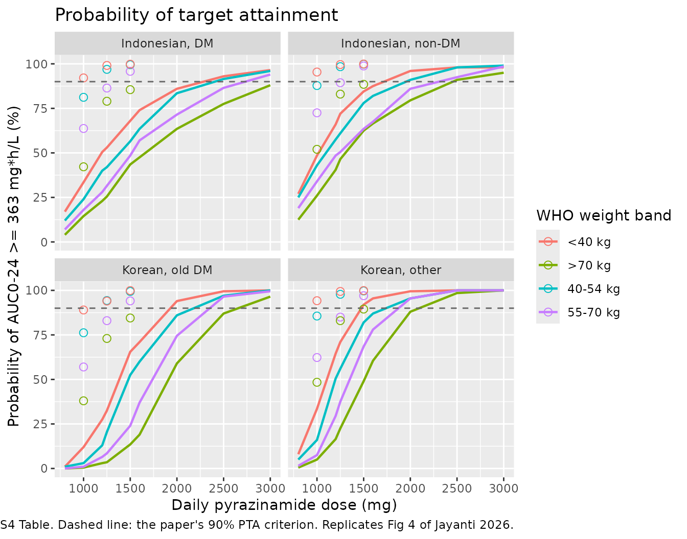
The published PTA tables are not reproducible from the published model, and the disagreement is in the source. The model’s attainment curves are markedly flatter and lower than S3/S4 Table at every band:
pta_cmp |>
  mutate(diff = pta - pta_pub) |>
  group_by(band) |>
  summarise(`Median model PTA (%)` = median(pta),
            `Median published PTA (%)` = median(pta_pub),
            `Median difference (points)` = median(diff),
            `Largest difference (points)` = diff[which.max(abs(diff))],
            .groups = "drop") |>
  rename("WHO weight band" = band) |>
knitr::kable(digits = 1, caption = "Model minus published probability of target attainment, over the 12 band-by-dose cells S4 Table reports.")| WHO weight band | Median model PTA (%) | Median published PTA (%) | Median difference (points) | Largest difference (points) |
|---|---|---|---|---|
| 40-54 kg | 47.0 | 97.3 | -46.4 | -76.3 |
| 55-70 kg | 34.0 | 85.7 | -49.4 | -77.0 |
| <40 kg | 56.0 | 99.2 | -43.4 | -81.0 |
| >70 kg | 22.2 | 81.0 | -44.5 | -72.0 |
The decisive check needs no model at all: the paper’s own S2 Table implies the same attainment this model does, and both disagree with S3 Table. S2 Table reports the Indonesian non-DM post-hoc AUC0-24 at 1,200 mg as a median of 388.6 mgh/L with an interquartile range of 318.1-515.4. Fitting a log-normal to those three published numbers and reading off the fraction above the paper’s own 363 mgh/L target gives an attainment that lands on top of the model’s, and nowhere near the 97.8% S3 Table prints for that stratum and dose.
# (a) This model, Indonesian non-DM, 40-54 kg band, 1,200 mg.
pta_model_cell <- pick("40-54 kg", "Indonesian, non-DM", 1200)

# (b) Implied by S2 Table's OWN post-hoc AUC0-24 distribution for the same
#     stratum at the same dose: log-normal through median 388.6 and IQR
#     318.1-515.4, evaluated at the paper's 363 mg*h/L target.
s2_med <- 388.6; s2_q1 <- 318.1; s2_q3 <- 515.4
s2_sdlog <- log(s2_q3 / s2_q1) / (2 * qnorm(0.75))
pta_from_s2 <- 100 * pnorm(log(s2_med / target_auc) / s2_sdlog)

# (c) As printed in S3 Table for the WHO 1,200 mg dose, 40-54 kg band.
pta_published <- 97.8

tibble::tibble(
  Source = c("This model", "Implied by S2 Table's own post-hoc AUC quartiles",
             "As printed in S3 Table"),
  `PTA (%)` = c(pta_model_cell, pta_from_s2, pta_published)
) |>
knitr::kable(digits = 1, caption = "Probability of AUC0-24 >= 363 mg*h/L for Indonesian non-diabetic patients in the 40-54 kg band at 1,200 mg, computed three ways.")| Source | PTA (%) |
|---|---|
| This model | 57.0 |
| Implied by S2 Table’s own post-hoc AUC quartiles | 57.6 |
| As printed in S3 Table | 97.8 |
# The model agrees with the paper's own post-hoc distribution far better than
# that distribution agrees with the paper's PTA table. This is the gate: it goes
# red if the model ever stops reproducing S2 Table, which is the claim being
# made -- it is NOT a gate on the S3 Table value, which is the documented
# deviation.
stopifnot(abs(pta_model_cell - pta_from_s2) < 15,
          abs(pta_from_s2 - pta_published) > 25)
Two further observations point the same way.
-
The published PTA barely differs between ethnicities, but
the model’s variances differ by a factor of four. Table 2 gives
the Indonesian clearance variance as 0.205 and the Korean as 0.05, a
factor of two in
omega. Two populations whose clearance spreads differ that much cannot produce the nearly superimposable attainment curves S3/S4 Table report – the<40 kgband at 800 mg is 70.4% for both ethnicities, to the decimal. -
The slope of the published dose-response implies a much
narrower spread than Table 2. Reading
omegaoff consecutive S4 Table doses in the 40-54 kg band gives about 0.23, which matches the Koreanomega(0.224) and not the Indonesian one (0.453).
Together these suggest the Monte Carlo behind S3/S4 Table did not use
the final model as Table 2 reports it – a single shared
omega, and possibly a different allometric reference, would
both push attainment up. No parameter was tuned to close the gap; the
model file follows Table 2, which is what S2 Table corroborates.
The paper’s qualitative dose ranking survives, and is what a user should take from the PTA analysis:
claims <- tibble::tribble(
  ~Claim, ~Model,
  "WHO 800 mg under-doses the <40 kg band (paper: 70.4%)",     pick("<40 kg", "Indonesian, non-DM", 800),
  "Raising <40 kg to 1,250 mg improves attainment",            pick("<40 kg", "Indonesian, non-DM", 1250),
  "Korean old DM attains less than Korean other, <40 kg 1,250 mg",
    pick("<40 kg", "Korean, old DM", 1250),
  "Indonesian DM attains less than Indonesian non-DM, 40-54 kg 1,250 mg",
    pick("40-54 kg", "Indonesian, DM", 1250)
)

# Directional claims only: magnitudes are the documented deviation above.
stopifnot(
  pick("<40 kg", "Indonesian, non-DM", 1250) > pick("<40 kg", "Indonesian, non-DM", 800),
  pick("<40 kg", "Korean, old DM", 1250)     < pick("<40 kg", "Korean, other", 1250),
  pick("40-54 kg", "Indonesian, DM", 1250)   < pick("40-54 kg", "Indonesian, non-DM", 1250),
  pick(">70 kg", "Indonesian, non-DM", 1000) < pick("<40 kg", "Indonesian, non-DM", 1000)
)

claims |>
  rename("Model PTA (%)" = Model) |>
knitr::kable(digits = 1, caption = "Directional claims from the paper's dose exploration, evaluated on the packaged model.")| Claim | Model PTA (%) |
|---|---|
| WHO 800 mg under-doses the <40 kg band (paper: 70.4%) | 30.5 |
| Raising <40 kg to 1,250 mg improves attainment | 63.5 |
| Korean old DM attains less than Korean other, <40 kg 1,250 mg | 27.0 |
| Indonesian DM attains less than Indonesian non-DM, 40-54 kg 1,250 mg | 49.0 |
Assumptions and deviations
- Lean-body-weight distribution. Table 1 reports medians and interquartile ranges by ethnicity but not a distributional form. Lean body weight is drawn log-normally, centred on the Table 1 medians, with the log-scale spread recovered from the Table 1 interquartile ranges and truncated to the range observed in the deposited dataset (32.45-68.17 kg). The paper does not report lean body weight by diabetes stratum, so both strata of an ethnicity share a distribution. For the weight-band PTA analysis the per-band lean body weight is taken from the deposited dataset instead, for the Boer-extrapolation reason given in that section.
- Post-hoc versus prior-predictive. S2 Table and Fig 3 report medians of individual Bayesian post-hoc estimates, each informed by that patient’s own concentrations and shrunk toward the typical value (35.9% and 56.9% shrinkage on the two clearance terms, 24.6% on volume). The simulation here is a prior-predictive draw from the population model, so it reproduces the centre of those distributions but is wider in the tails by construction.
- Subgroup sizes. Simulated arms are equal-sized (200 each). The real subgroups were very unequal – 13 Korean old-DM patients against 147 others, 55 Indonesian diabetic against 105 non-diabetic – so the published medians for the small strata carry far wider uncertainty than the simulated ones.
-
Dose and steady state. Doses are 1,200 mg once
daily to match the normalising dose of S2 Table and Fig 3; the real
cohort received 500-2,000 mg, most commonly 1,500 mg (42.8%). Seven
daily doses are simulated and NCA is taken over the seventh interval,
which is well past steady state for a ~10 h half-life. The deposited
dataset codes every dose record as
SS = 1withII = 24, confirming the paper fitted steady-state data. -
IIV on Ka is omitted, not encoded as a zero-variance
eta. Table 2 reports
omega^2; Ka (%)as0 (FIX). Declaringetalka ~ fixed(0)would put a structural zero on the OMEGA diagonal and make it singular, which fails at the Cholesky factorisation during simulation. Omitting the eta is the faithful encoding of a variance fixed to zero. -
Covariates screened but not retained (total body
weight, continuous age, height, sex, albumin, AST, ALT, total bilirubin,
blood urea nitrogen, serum creatinine, eGFR, liver disease and
ethnicity-as-a-covariate) are recorded in the model file’s
covariatesDataExcludedmetadata rather thancovariateData, since none is referenced inmodel(). Albumin and AST are the notable cases: both were significant univariately and were dropped for large standard errors. -
All parameter values come from the paper’s Table 2,
including its footnote d. No value was taken from author
correspondence, figure digitisation, or an upstream model. The deposited
dataset (S2 File) was used only to resolve covariate coding –
the age threshold, the ethnicity code, the sex code and the
OLDDMdefinition – and to characterise lean body weight per weight band for the PTA section; no parameter estimate came from it.
Errata and internal inconsistencies in the source
-
Published PTA tables are not reproducible from the published
model. See the target-attainment section; S3/S4 Table imply a
clearance spread near half of the Indonesian
omegareported in Table 2 and are inconsistent with the paper’s own S2 Table exposure quartiles. The model file follows Table 2. -
The 45 kg allometric reference appears only in the Table 2
footnote, which PDF-to-markdown conversion drops (a
layout-preserving text extraction and the rendered table image both keep
it). Recorded here and in the model file’s
LBMcovariate notes so it is not re-derived. -
The age threshold is printed inconsistently. Table
1’s row header and the S3/S4 Table footnotes say “Age > 60 years
old”; Methods, Results and the Fig 3 caption say “>= 60 years”. The
deposited dataset settles it – the
OLDcolumn is 0 for ages 17-59 and 1 for ages 60-80 – so the inclusive form is correct and the model usesAGE_GE60. - Vd/F and Ka are quoted differently in the Discussion than in Table 2. The Discussion says “The Vd/F (53.4 L) and Ka (2.1 h-1) values of our model”, while Table 2 gives 52.8 L and 2.0 1/h with bootstrap medians of 52.7 and 2.05. The model uses the Table 2 values, per the standing rule that the final parameter table takes precedence over prose.
- The Abstract mislabels the two clearance typical values. It reads “There were 23% and 26% increases in apparent clearance (CL/F) of Indonesian patients with DM (CL/F 3.18 L/h) and Korean patients aged > 60 years with DM (CL/F 3.5)”, attaching the reference (non-diabetic) clearances to the diabetic groups. The Results give the diabetic values correctly as 3.88 and 4.38 L/h.
- The DM coefficients are printed to different precision in different places. Table 2 gives 0.23 and 0.26; the Results text gives 0.226 and 0.252. The model uses the Table 2 values; the difference moves the diabetic clearances by under 1%.
- Lean body weight exceeds total body weight for 12 of the 300 deposited patients (up to a ratio of 1.14), because the Boer equation is extrapolated outside its validity for low-BMI tuberculosis patients. This is a property of the covariate definition the paper adopted, not a transcription error, but it means lean body weight should not be reconstructed from independently sampled weight and height at the low end of the weight range.
- The deposited dataset is slightly smaller than the modelled cohort – 300 subjects and 404 quantifiable records against the 320 subjects and 407 concentrations described in the Results. The parameter estimates come from the paper, so this affects only the covariate-coding checks above.
- The published correction (PLoS One 2026;21(4):e0347490) revises the funding statement only and changes no model value.