Copanlisib (Morcos 2023)
Source:vignettes/articles/Morcos_2023_copanlisib.Rmd
Morcos_2023_copanlisib.RmdModel and source
#> ℹ parameter labels from comments will be replaced by 'label()'Citation: Morcos PN, Moss J, Austin R, Hiemeyer F, Zinzani PL, Beckert V, Mongay Soler L, Childs BH, Garmann D. Copanlisib population pharmacokinetics from phase I-III studies and exposure-response relationships in combination with rituximab. CPT Pharmacometrics Syst Pharmacol. 2023;12(11):1666-1686. doi:10.1002/psp4.13000.
Description: Three-compartment population PK model for intravenous copanlisib in adults with advanced solid tumors or non-Hodgkin lymphoma, pooled across nine phase I-III studies (n = 712), with categorical covariate effects of rifampicin and itraconazole comedication, sex, hepatic impairment, Japanese region and CHRONOS-3 study membership on clearance and central volume, and an infusion-time / study-phase stratified log-additive residual error
Article: https://doi.org/10.1002/psp4.13000
Supplement (Tables S1-S3, Figures S1-S4): https://doi.org/10.1002/psp4.13000 (Supporting Information, file
PSP4-12-1666-s001.docx)
Copanlisib is an intravenous pan-class-I PI3K inhibitor approved for relapsed follicular lymphoma. Morcos 2023 pooled 5958 plasma concentrations from 712 patients across nine phase I-III studies into a single population PK model, and then used that model’s individual exposure predictions to drive exposure-response analyses in the phase III CHRONOS-3 trial.
The packaged model is the paper’s final population PK covariate model (Table 2). The exposure-response layer is not packaged; see Assumptions and deviations for why.
Population
| Field | Value |
|---|---|
| species | human |
| n_subjects | 712 |
| n_studies | 9 |
| n_observations | 5958 |
| age_range | 20-91 years |
| age_median | 63 years |
| weight_range | 41.1-165 kg |
| weight_median | 70.0 kg |
| sex_female_pct | 52.4 |
| disease_state | advanced solid tumors, aggressive non-Hodgkin lymphoma, or indolent non-Hodgkin lymphoma (chiefly relapsed follicular lymphoma); one phase I study also enrolled healthy participants alongside hepatic- and renal-impairment cohorts |
| dose_range | 0.1-1.2 mg/kg or 12-60 mg flat, given as a 1-h intravenous infusion on days 1, 8 and 15 of a 28-day cycle (3 weeks on / 1 week off); the approved and phase III regimen is 60 mg flat |
| regions | Europe (49.3%), North America (20.6%), mainland China (9.8%), Japan (8.6%), other Asia (3.9%), other (7.7%) |
| hepatic_function | 84.1% normal, 14.9% mild, 0.4% moderate, 0.6% severe (NCI ODWG) |
| renal_function | 46.8% normal, 40.2% mild, 11.8% moderate, 1.3% severe (NCI criteria) |
| albumin_median | 4.14 g/dL (range 1.6-6.5) |
| egfr_median | 87.9 mL/min (range 13.64-155.91) |
| co_medication | rituximab 375 mg/m2 in study 17067 (CHRONOS-3) only; rifampicin or itraconazole in the dedicated DDI study 16270 only |
| notes | Baseline demographics are Morcos 2023 Table 1, column ‘Pooled PopPK analyses’; the per-study designs, dosing regimens and PK sampling schedules are Table S1. The nine studies are 12871, 15205, 16270, 16349 (parts A and B, CHRONOS-1), 16790, 16866, 17067 (CHRONOS-3), 17792 and 18041. Concentrations were measured by validated LC/MS with an LLOQ of 2 ng/mL; 276 of 5958 observations were below that limit and were handled with the Beal M3 method, which is a likelihood-estimation device and has no counterpart in a forward simulation. |
The pooled analysis population is 712 adults with advanced solid tumors or non-Hodgkin lymphoma, median age 63 years (range 20-91), median body weight 70.0 kg (range 41.1-165), 52.4% female (Morcos 2023 Table 1). Copanlisib was given as a 1-h intravenous infusion on days 1, 8 and 15 of a 28-day cycle, at 0.1-1.2 mg/kg in the dose-escalation studies and at a 60 mg flat dose in the phase II and phase III studies. Concentrations were measured by validated LC/MS with an LLOQ of 2 ng/mL; 276 of 5958 observations were below that limit and were handled with the Beal M3 method.
The simulations below reproduce the CHRONOS-3
subpopulation (Bayer study 17067, NCT02367040), because that is the
cohort for which the paper publishes exposure percentiles. Its baseline
distribution comes from the Study 17067 column of Table 1
(n = 447): 47.7% female, 15.7% with any hepatic impairment (15.2% mild +
0.4% moderate), and 7.8% enrolled at Japanese sites.
Source trace
Every ini() entry in
inst/modeldb/specificDrugs/Morcos_2023_copanlisib.R carries
an in-file comment naming its source. They are collected here for
review.
| Equation / parameter | Value | Source location |
|---|---|---|
| Three-compartment IV disposition, first-order elimination from central | n/a | Results, “PopPK meta-analyses”; schematic Figure S1 |
Categorical covariate form
P = Ptv * (1 + N1*th1 + N2*th2 + ...) * exp(eta)
|
n/a | Methods, “Copanlisib PopPK modeling” (third displayed equation) |
lcl (CL) |
22.2 L/h | Table 2, CL pop (RSE 3.18%, 95% CI 20.8-23.5) |
lvc (V1) |
92.1 L | Table 2, V1 pop (RSE 7.47%, 95% CI 78.6-106) |
lq (Q2) |
79.3 L/h | Table 2, Q2 (RSE 1.58%) |
lvp (V2) |
508 L | Table 2, V2 (RSE 2.54%) |
lq2 (Q3) |
7.34 L/h | Table 2, Q3 (RSE 6.96%) |
lvp2 (V3) |
522 L | Table 2, V3 (RSE 4.26%) |
e_conmed_rifampicin_cl |
1.91 | Table 2 Theta RIFCL; Results “increased CL by
191%” |
e_conmed_itraconazole_cl |
-0.361 | Table 2 Theta ITRACL; Results “decreased CL by
36.1%” |
e_study_chronos3_cl |
-0.184 | Table 2 Theta 17067CL; Results “18.4% lower CL” |
e_sexf_cl |
-0.167 | Table 2 Theta SEXCL; Results “females had 16.7% lower
CL” |
e_hepimp_cl |
-0.192 | Table 2 Theta NCICL; Results “19.2% lower CL” |
e_region_japan_cl |
-0.204 | Table 2 Theta JAPCL; Results “Japan had 20.4% lower
CL” |
e_sexf_vc |
-0.429 | Table 2 Theta SEXV1; Results “females had 42.9% lower
V1” |
e_conmed_rifampicin_vc |
1.08 | Table 2 Theta RIFV1; Results “rifampin increased V1 by
108%” |
etalcl variance |
0.124 | Table 2 OMEGA on CL pop (CV 36.3%, shrinkage
22.5%) |
etalvc variance |
0.846 | Table 2 OMEGA on V1 pop (CV 115%, shrinkage 27.3%) |
expSd_early |
sqrt(5.10) = 2.2583 | Table 2 SIGMA, “first 20 min of an infusion” (CV 1280%) |
expSd_phase12 |
sqrt(0.176) = 0.4195 | Table 2 SIGMA, “phase I and phase II … after first 20 min” (CV 43.9%) |
expSd_phase3 |
sqrt(0.632) = 0.7950 | Table 2 SIGMA, “phase III for study 17067 … after first 20 min” (CV 93.8%) |
Log-additive residual = lnorm()
|
n/a | Table 2 footnote g |
| Reference patient (all indicators 0) | n/a | Table 2 footnotes d and e |
The paper’s reference patient is a male, in a non-Japanese phase I or phase II study, without rifampicin or itraconazole comedication, with normal hepatic function. Setting every covariate indicator to 0 in the packaged model recovers that patient exactly.
Variance components reproduce Table 2
Table 2 reports each variance twice: as omega^2 /
sigma^2, and as a percent CV derived by
100 * sqrt(exp(v) - 1) (footnotes f and g). The packaged
model stores standard deviations, so back-transforming them must
regenerate the published CV column. This is a deterministic identity -
no simulation, no cohort - so it is asserted tightly.
iniDf <- ui$iniDf

get_est <- function(nm) {
  v <- iniDf$est[iniDf$name == nm]
  stopifnot(length(v) == 1L)
  v
}

cv_pct <- function(variance) 100 * sqrt(exp(variance) - 1)

variance_check <- tibble::tibble(
  Component = c("IIV on CL", "IIV on V1",
                "Residual, first 20 min of infusion",
                "Residual, phase I/II beyond 20 min",
                "Residual, phase III beyond 20 min"),
  `Table 2 variance` = c(0.124, 0.846, 5.10, 0.176, 0.632),
  `Model value` = c(
    get_est("etalcl"),           # stored as a variance
    get_est("etalvc"),           # stored as a variance
    get_est("expSd_early")^2,    # stored as a log-scale SD
    get_est("expSd_phase12")^2,
    get_est("expSd_phase3")^2
  ),
  `Table 2 CV (%)` = c(36.3, 115, 1280, 43.9, 93.8)
) |>
  mutate(
    `Model CV (%)` = cv_pct(`Model value`),
    `CV rel. diff (%)` = 100 * (`Model CV (%)` - `Table 2 CV (%)`) / `Table 2 CV (%)`
  )

knitr::kable(variance_check, digits = c(0, 4, 4, 1, 1, 2),
caption = "Back-transformed variance components against the published CV column of Morcos 2023 Table 2.")| Component | Table 2 variance | Model value | Table 2 CV (%) | Model CV (%) | CV rel. diff (%) |
|---|---|---|---|---|---|
| IIV on CL | 0.124 | 0.1240 | 36.3 | 36.3 | 0.09 |
| IIV on V1 | 0.846 | 0.8460 | 115.0 | 115.3 | 0.29 |
| Residual, first 20 min of infusion | 5.100 | 5.0999 | 1280.0 | 1276.7 | -0.25 |
| Residual, phase I/II beyond 20 min | 0.176 | 0.1760 | 43.9 | 43.9 | -0.08 |
| Residual, phase III beyond 20 min | 0.632 | 0.6320 | 93.8 | 93.9 | 0.09 |
Covariate effects reproduce Table 2
Each of the eight retained covariates is a binary indicator entering
as a multiplicative (1 + theta) factor. Solving the
typical-value model (zeroRe()) once per single-covariate
configuration and dividing each clearance by the reference patient’s
clearance must return 1 + theta exactly.
mod <- readModelDb("Morcos_2023_copanlisib")
mod_typ <- rxode2::zeroRe(mod)
#> ℹ parameter labels from comments will be replaced by 'label()'
#> Warning: No sigma parameters in the model

cov_names <- c("SEXF", "HEPIMP", "REGION_JAPAN", "CONMED_RIFAMPICIN",
               "CONMED_ITRACONAZOLE", "STUDY_CHRONOS3")

# One subject per configuration: subject 1 is the reference patient (all
# indicators 0), then one subject per covariate turned on alone.
probe_cov <- matrix(0, nrow = 1 + length(cov_names), ncol = length(cov_names),
                    dimnames = list(NULL, cov_names))
for (i in seq_along(cov_names)) probe_cov[i + 1L, cov_names[i]] <- 1

probe_subj <- tibble::as_tibble(probe_cov) |>
  mutate(
    id = seq_len(n()),
    config = c("Reference (all indicators 0)",
               "Female", "Any hepatic impairment", "Japan",
               "Rifampicin", "Itraconazole", "CHRONOS-3")
  )

# 60 mg over a 1-h infusion into `central`; observations on the ODE state.
probe_dose <- probe_subj |>
  mutate(time = 0, amt = 60, evid = 1L, cmt = "central", rate = 60)
probe_obs <- probe_subj |>
  tidyr::crossing(time = c(0.5, 1, 2)) |>
  mutate(amt = NA_real_, evid = 0L, cmt = "central", rate = NA_real_)

probe_ev <- bind_rows(probe_dose, probe_obs) |>
  select(id, time, amt, evid, cmt, rate, all_of(cov_names), config) |>
  arrange(id, time, desc(evid))

probe_sim <- rxode2::rxSolve(mod_typ, events = probe_ev, keep = "config") |>
  as.data.frame()
#> ℹ omega/sigma items treated as zero: 'etalcl', 'etalvc'
#> Warning: multi-subject simulation without without 'omega'

probe_par <- probe_sim |>
  group_by(id, config) |>
  summarise(cl = unique(round(cl, 10)), vc = unique(round(vc, 10)), .groups = "drop")

ref_cl <- probe_par$cl[probe_par$config == "Reference (all indicators 0)"]
ref_vc <- probe_par$vc[probe_par$config == "Reference (all indicators 0)"]

cov_check <- probe_par |>
  filter(config != "Reference (all indicators 0)") |>
  mutate(
    `CL factor` = cl / ref_cl,
    `V1 factor` = vc / ref_vc
  ) |>
  select(Configuration = config, `CL factor`, `V1 factor`) |>
  mutate(
    `Expected CL factor` = 1 + c(-0.167, -0.192, -0.204, 1.91, -0.361, -0.184),
    `Expected V1 factor` = 1 + c(-0.429, 0, 0, 1.08, 0, 0)
  )

knitr::kable(cov_check, digits = 4,
caption = "Typical-value covariate factors against 1 + theta from Morcos 2023 Table 2.")| Configuration | CL factor | V1 factor | Expected CL factor | Expected V1 factor |
|---|---|---|---|---|
| Female | 0.833 | 0.571 | 0.833 | 0.571 |
| Any hepatic impairment | 0.808 | 1.000 | 0.808 | 1.000 |
| Japan | 0.796 | 1.000 | 0.796 | 1.000 |
| Rifampicin | 2.910 | 2.080 | 2.910 | 2.080 |
| Itraconazole | 0.639 | 1.000 | 0.639 | 1.000 |
| CHRONOS-3 | 0.816 | 1.000 | 0.816 | 1.000 |
# Deterministic algebra; the only slack is double-precision round-off.
stopifnot(
  max(abs(cov_check$`CL factor` - cov_check$`Expected CL factor`)) < 1e-8,
  max(abs(cov_check$`V1 factor` - cov_check$`Expected V1 factor`)) < 1e-8
)

# The reference patient's typical values must be Table 2's CL pop and V1 pop.
stopifnot(
  abs(ref_cl - 22.2) < 1e-8,
  abs(ref_vc - 92.1) < 1e-8
)
Disposition of a single 60 mg dose
Before turning to the intermittent regimen, the typical-value profile
after one 60 mg infusion establishes the terminal half-life and confirms
the fundamental identity AUC(0-inf) = dose / CL.
sd_times <- sort(unique(c(
  seq(0, 4, by = 0.05), seq(4, 24, by = 0.25),
  seq(24, 168, by = 2), seq(168, 1008, by = 8)
)))

sd_ev <- bind_rows(
  tibble::tibble(id = 1L, time = 0, amt = 60, evid = 1L, cmt = "central", rate = 60),
  tibble::tibble(id = 1L, time = sd_times, amt = NA_real_, evid = 0L,
                 cmt = "central", rate = NA_real_)
) |>
  mutate(SEXF = 0, HEPIMP = 0, REGION_JAPAN = 0, CONMED_RIFAMPICIN = 0,
         CONMED_ITRACONAZOLE = 0, STUDY_CHRONOS3 = 0) |>
  arrange(time, desc(evid))

sd_sim <- rxode2::rxSolve(mod_typ, events = sd_ev) |> as.data.frame()
#> ℹ omega/sigma items treated as zero: 'etalcl', 'etalvc'

# rxSolve DROPS the id column entirely when the event table holds a single
# subject, and PKNCA's grouping formula below needs it. Restore it rather than
# assuming it is there.
if (is.null(sd_sim$id)) sd_sim$id <- 1L

# Concentrations must stay non-negative; a negative far tail would make
# PKNCA's log-down trapezoid produce NaN.
stopifnot(all(sd_sim$Cc >= 0))

sd_sim |>
  filter(time > 0) |>
  ggplot(aes(time, Cc)) +
  geom_line(linewidth = 0.7) +
  scale_x_continuous(breaks = seq(0, 1008, by = 168)) +
  scale_y_log10() +
  labs(
    x = "Time (h)", y = "Copanlisib concentration (mg/L)",
    title = "Typical-value profile, single 60 mg 1-h intravenous infusion",
    caption = "Three-compartment disposition of Morcos 2023 Table 2, reference patient."
  ) +
  theme_bw()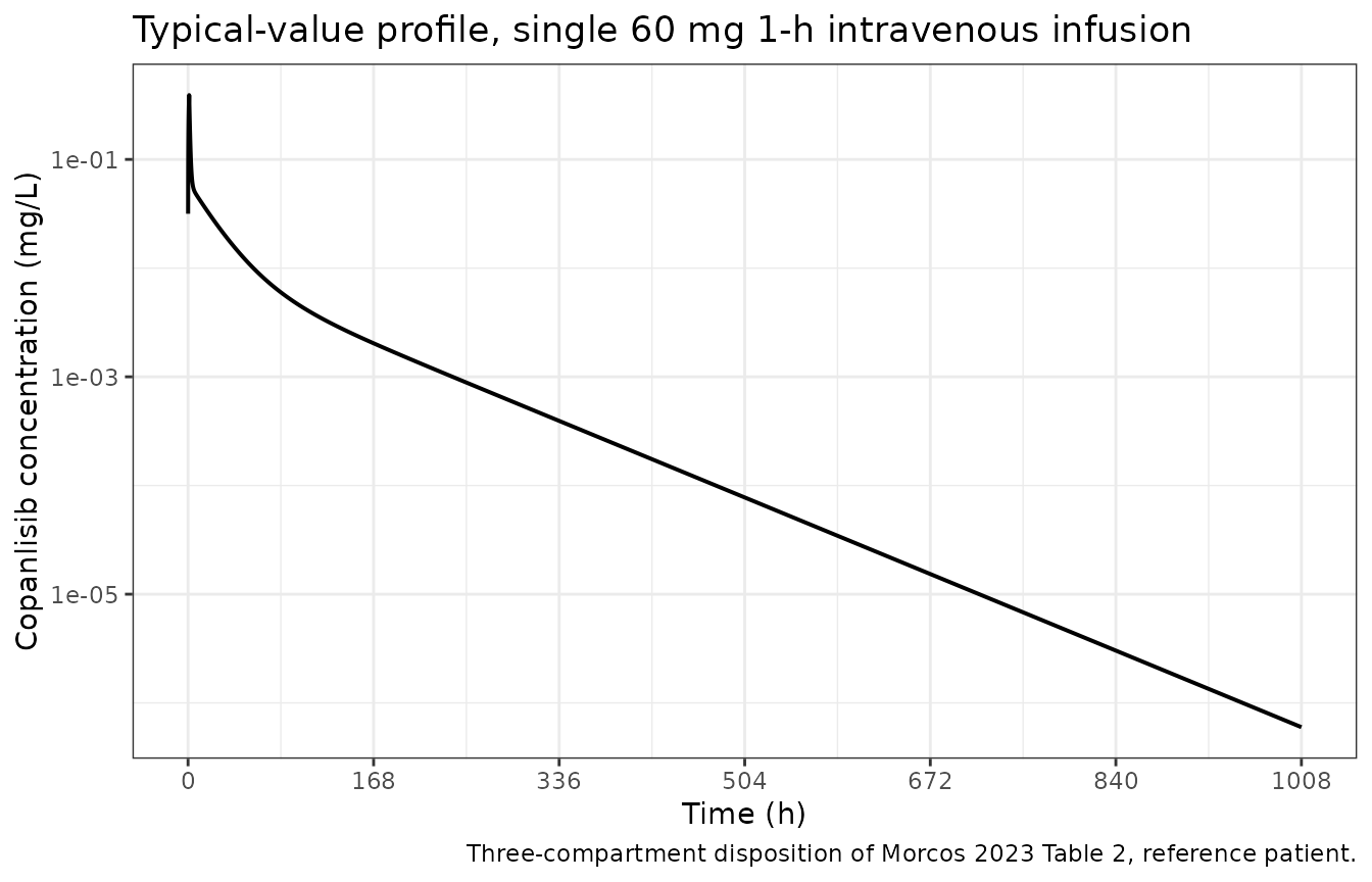
sd_conc <- sd_sim |>
  filter(!is.na(Cc)) |>
  select(id, time, Cc) |>
  mutate(treatment = "60 mg single dose")

sd_dose <- tibble::tibble(id = 1L, time = 0, amt = 60,
                          treatment = "60 mg single dose")

sd_res <- PKNCA::pk.nca(PKNCA::PKNCAdata(
  PKNCA::PKNCAconc(as.data.frame(sd_conc), Cc ~ time | treatment + id,
                   concu = "mg/L", timeu = "h"),
  PKNCA::PKNCAdose(as.data.frame(sd_dose), amt ~ time | treatment + id,
                   doseu = "mg"),
  intervals = data.frame(start = 0, end = Inf,
                         cmax = TRUE, tmax = TRUE,
                         auclast = TRUE, aucinf.obs = TRUE, half.life = TRUE)
))

sd_tbl <- as.data.frame(sd_res$result) |>
  select(PPTESTCD, PPORRES) |>
  tidyr::pivot_wider(names_from = PPTESTCD, values_from = PPORRES)

knitr::kable(
  sd_tbl |>
    dplyr::select(cmax, tmax, auclast, aucinf.obs, half.life) |>
    dplyr::rename(
      "Cmax (mg/L)"         = cmax,
      "Tmax (h)"            = tmax,
      "AUClast (mg*h/L)"    = auclast,
      "AUC0-inf (mg*h/L)"   = aucinf.obs,
      "Terminal t1/2 (h)"   = half.life
    ),
  digits = 3,
  caption = "PKNCA on the typical-value single-dose profile."
)| Cmax (mg/L) | Tmax (h) | AUClast (mg*h/L) | AUC0-inf (mg*h/L) | Terminal t1/2 (h) |
|---|---|---|---|---|
| 0.39 | 1 | 2.703 | 2.703 | 71.263 |
auc_inf <- sd_tbl$aucinf.obs
thalf   <- sd_tbl$half.life

# Fail loudly rather than silently reporting NA downstream: an NA half-life
# would mean PKNCA found too few post-peak points to fit lambda-z, which is a
# problem with the sampling grid above, not a property of the model.
stopifnot(is.finite(auc_inf), is.finite(thalf))

# Internal identity: for a linear model with no IIV and no residual error,
# AUC(0-inf) is exactly dose / CL. The only error is trapezoidal.
stopifnot(abs(auc_inf - 60 / 22.2) / (60 / 22.2) < 0.01)

# The 1008 h window is many terminal half-lives long, so AUClast has
# effectively converged onto AUC(0-inf); assert >= because auclast can only
# undershoot aucinf.obs.
stopifnot(sd_tbl$auclast <= auc_inf,
          (auc_inf - sd_tbl$auclast) / auc_inf < 0.01)
The model’s terminal half-life is 71.3 h. Morcos 2023’s Introduction quotes “a half-life of around 38 h” at the maximum tolerated dose, but that figure comes from the earlier phase I analysis (reference 5 of the paper) and is a reported rather than a modelled value; the present three-compartment model, which resolves a deep peripheral compartment with Q3 = 7.34 L/h and V3 = 522 L, necessarily supports a longer terminal slope. The paper itself reports no half-life for this model, so this is a cross-analysis observation, not a discrepancy - it is recorded in Assumptions and deviations and is deliberately excluded from the assertion gate.
Virtual CHRONOS-3 cohort
# set.seed() seeds R's RNG, which draws the covariate configuration below. It
# does NOT seed rxode2's simulation RNG, and rxode2 partitions its streams per
# solver thread -- so the etas drawn downstream differ between a 2-core CI
# runner and a many-thread workstation. Every assertion below is therefore
# written to hold for any cohort this model can produce.
set.seed(20231101)

n_sub <- 200L   # cap is 200 participants per arm

# Baseline proportions from Morcos 2023 Table 1, column "Study 17067" (n = 447,
# the CHRONOS-3 exposure-response population): 213/447 = 47.7% female;
# (68 + 2)/447 = 15.7% with any hepatic impairment; 35/447 = 7.8% Japan.
#
# Subgroup membership is assigned with EXACT counts rather than rbinom(), so
# every subgroup has a fixed, reproducible size on any machine. With only ~8%
# Japan prevalence, binomial assignment would let the Japanese subgroup range
# from about 8 to 25 subjects between runs, and the subgroup geometric mean
# asserted below would inherit that extra noise for no benefit.
assign_exact <- function(n, k) {
  v <- integer(n)
  v[sample.int(n, k)] <- 1L
  v
}

subj <- tibble::tibble(
  id                  = seq_len(n_sub),
  SEXF                = assign_exact(n_sub, 95L),   # 47.7% of 200 = 95.4
  HEPIMP              = assign_exact(n_sub, 31L),   # 15.7% of 200 = 31.4
  REGION_JAPAN        = assign_exact(n_sub, 16L),   #  7.8% of 200 = 15.6
  CONMED_RIFAMPICIN   = 0,   # given only in the dedicated DDI study 16270
  CONMED_ITRACONAZOLE = 0,   # given only in the dedicated DDI study 16270
  STUDY_CHRONOS3      = 1,
  treatment           = "Copanlisib 60 mg, days 1/8/15"
)

stopifnot(sum(subj$SEXF) == 95L, sum(subj$HEPIMP) == 31L,
          sum(subj$REGION_JAPAN) == 16L)

# AUC(0-168)nd is defined in Methods, "Determination of copanlisib exposure
# metrics": the AUC from 0 to 168 h AFTER THE THIRD 60 mg nominal dose in a
# sequence of three doses of 60 mg each one week apart. So dose at 0, 168 and
# 336 h and integrate over [336, 504].
dose_times <- c(0, 168, 336)
auc_start  <- 336
auc_end    <- 504

# Dense sampling around each infusion plus a regular backbone, so the
# trapezoidal AUC over [336, 504] resolves the distribution phase.
fine <- c(0, 0.25, 0.5, 0.75, 1, 1.1, 1.25, 1.5, 2, 2.5, 3, 4, 5, 6, 8, 11, 14, 18, 24)
obs_times <- sort(unique(c(
  as.vector(outer(dose_times, fine, "+")),
  seq(0, auc_end, by = 4),
  auc_start, auc_end
)))
obs_times <- obs_times[obs_times <= auc_end]

events <- bind_rows(
  subj |>
    tidyr::crossing(time = dose_times) |>
    mutate(amt = 60, evid = 1L, cmt = "central", rate = 60),
  subj |>
    tidyr::crossing(time = obs_times) |>
    mutate(amt = NA_real_, evid = 0L, cmt = "central", rate = NA_real_)
) |>
  select(id, time, amt, evid, cmt, rate,
         SEXF, HEPIMP, REGION_JAPAN, CONMED_RIFAMPICIN, CONMED_ITRACONAZOLE,
         STUDY_CHRONOS3, treatment) |>
  arrange(id, time, desc(evid))

stopifnot(!anyDuplicated(unique(events[, c("id", "time", "evid")])))
Simulation
sim <- rxode2::rxSolve(
  mod, events = events,
  keep = c("SEXF", "HEPIMP", "REGION_JAPAN", "treatment")
) |>
  as.data.frame()
#> ℹ parameter labels from comments will be replaced by 'label()'

# rxSolve returns Cc (== ipredSim, NO residual error) alongside `sim` (which
# DOES carry the residual). Everything below deliberately uses Cc: the
# published exposure metrics are model-predicted AUCs, not assayed values.
stopifnot(isTRUE(all.equal(sim$Cc, sim$ipredSim)))
stopifnot(all(sim$Cc >= 0), !anyNA(sim$Cc))
# Companion to Figure 1b of Morcos 2023 (prediction-corrected VPC of copanlisib
# PK in CHRONOS-3). Shown here over the third dosing interval, where the
# published AUC(0-168)nd is defined.
sim |>
  filter(time >= auc_start, time <= auc_end) |>
  mutate(tad = time - auc_start) |>
  group_by(tad) |>
  summarise(
    Q05 = quantile(Cc, 0.05),
    Q50 = quantile(Cc, 0.50),
    Q95 = quantile(Cc, 0.95),
    .groups = "drop"
  ) |>
  filter(tad > 0) |>
  ggplot(aes(tad, Q50)) +
  geom_ribbon(aes(ymin = Q05, ymax = Q95), alpha = 0.25) +
  geom_line(linewidth = 0.7) +
  scale_x_continuous(breaks = seq(0, 168, by = 24)) +
  scale_y_log10() +
  labs(
    x = "Time after third dose (h)", y = "Copanlisib concentration (mg/L)",
    title = "Simulated CHRONOS-3 exposure over the third dosing interval",
    caption = paste("Median with 5th-95th percentile band, n =", n_sub,
                    "virtual patients. Companion to Figure 1b of Morcos 2023.")
  ) +
  theme_bw()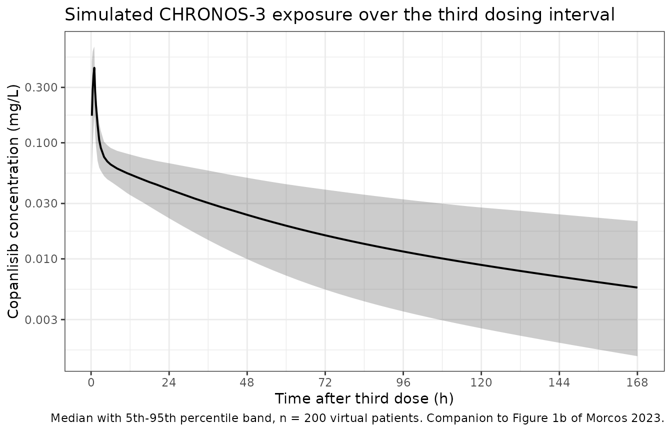
PKNCA validation
# Only !is.na(Cc) -- adding time > 0 or Cc > 0 would drop the anchor row that
# PKNCA needs at the start of the interval.
sim_nca <- sim |>
  filter(!is.na(Cc)) |>
  select(id, time, Cc, treatment)

# Guarantee a time-zero row per subject. This is an intravenous infusion, so
# the pre-dose concentration is 0.
sim_nca <- bind_rows(
  sim_nca,
  sim_nca |> distinct(id, treatment) |> mutate(time = 0, Cc = 0)
) |>
  distinct(id, treatment, time, .keep_all = TRUE) |>
  arrange(id, treatment, time)

conc_obj <- PKNCA::PKNCAconc(
  as.data.frame(sim_nca), Cc ~ time | treatment + id,
  concu = "mg/L", timeu = "h"
)

dose_df <- events |>
  filter(evid == 1L) |>
  select(id, time, amt, treatment)

dose_obj <- PKNCA::PKNCAdose(
  as.data.frame(dose_df), amt ~ time | treatment + id, doseu = "mg"
)

# AUC(0-168)nd = AUC over the interval that follows the third 60 mg dose.
intervals <- data.frame(
  start   = auc_start,
  end     = auc_end,
  cmax    = TRUE,
  tmax    = TRUE,
  auclast = TRUE,
  cav     = TRUE
)

nca_res <- PKNCA::pk.nca(PKNCA::PKNCAdata(conc_obj, dose_obj, intervals = intervals))

nca_tbl <- as.data.frame(nca_res$result) |>
  select(id, PPTESTCD, PPORRES) |>
  tidyr::pivot_wider(names_from = PPTESTCD, values_from = PPORRES)

# Convert the model's mg/L*h onto the paper's ug*h/L (1 mg/L = 1000 ug/L).
nca_tbl <- nca_tbl |> mutate(auc_ug_h_L = auclast * 1000)

auc_q <- quantile(nca_tbl$auc_ug_h_L, c(0.05, 0.50, 0.95))
Comparison against published exposure
Morcos 2023 reports AUC(0-168)nd for copanlisib-treated CHRONOS-3 patients in two places that agree with each other: Figure 3b prints a median of 3720 ugh/L with 5th-95th percentiles of 2650-5770, and the Discussion gives “the fifth and 95th percentiles of AUC[0-168]nd in CHRONOS-3 were 2647 and 5766 ngh/mL” (1 ng/mL = 1 ug/L, so the units are the same).
# AUC(0-168)nd is the ONLY NCA quantity this paper publishes for the model.
# Cmax and Tmax are never reported, and the paper's Cavg,2wk / Cavg,4wk /
# Cavg,8wk medians (13.9 / 13.8 / 13.1 ug/L, Figure 3b) are moving averages
# over each patient's ACTUAL dosing history -- which includes the week off
# every cycle and the dose interruptions that 75.2% of CHRONOS-3 patients
# experienced -- so they are not comparable to a nominal three-dose schedule
# and are deliberately excluded from this table.
published <- tibble::tibble(
  treatment = "Copanlisib 60 mg, days 1/8/15",
  auclast   = 3.720      # 3720 ug*h/L (Figure 3b) expressed in mg*h/L
)

cmp <- nlmixr2lib::ncaComparisonTable(
  simulated     = nca_res,
  reference     = published,
  by            = "treatment",
  params        = "auclast",
  units         = c(auclast = "mg*h/L"),
  tolerance_pct = 20
)

knitr::kable(
  cmp,
  caption = "Simulated AUC(0-168)nd (median of 200 virtual CHRONOS-3 patients) vs. Morcos 2023 Figure 3b. * differs from reference by >20%."
)| NCA parameter | treatment | Reference | Simulated | % diff |
|---|---|---|---|---|
| AUClast (mg*h/L) | Copanlisib 60 mg, days 1/8/15 | 3.72 | 3.86 | +3.8% |
exposure_check <- tibble::tibble(
  Statistic   = c("5th percentile", "Median", "95th percentile"),
  `Published (ug*h/L)` = c(2650, 3720, 5770),
  `Simulated (ug*h/L)` = as.numeric(auc_q)
) |>
  mutate(`Rel. diff (%)` = 100 * (`Simulated (ug*h/L)` - `Published (ug*h/L)`) /
           `Published (ug*h/L)`)

knitr::kable(exposure_check, digits = c(0, 0, 0, 1),
caption = "AUC(0-168)nd distribution against Morcos 2023 Figure 3b.")| Statistic | Published (ug*h/L) | Simulated (ug*h/L) | Rel. diff (%) |
|---|---|---|---|
| 5th percentile | 2650 | 2081 | -21.5 |
| Median | 3720 | 3863 | 3.8 |
| 95th percentile | 5770 | 7652 | 32.6 |
med_pct <- exposure_check$`Rel. diff (%)`[exposure_check$Statistic == "Median"]The median is the structural check, and it is the one asserted tightly: a mis-transcribed clearance, dose, covariate coefficient or unit moves the whole distribution by tens of percent.
# AUC(0-168)nd = dose / CL to better than 1% (by superposition the interval
# spans the whole of a single dose's disposition), so the median AUC is pinned
# by the median individual clearance. Subgroup sizes are fixed by construction,
# so the only noise left is the eta draw: the sample median of 200 log-normal
# draws with sigma = sqrt(0.124) = 0.352 has a log-scale standard error of
# 1.2533 * 0.352 / sqrt(200) = 0.031, i.e. +/- 9.4% at three standard errors.
# 15% therefore sits outside the achievable noise while still going red on any
# structural error worth catching: dropping the -18.4% CHRONOS-3 clearance
# effect alone moves the median by 22.5%, and a unit or dose error moves it by
# orders of magnitude.
stopifnot(abs(med_pct) < 15)
The tails are deliberately not gated, and the table above shows why: the simulated 5th-95th spread is wider than the published one. That is expected and is not a transcription problem. The published percentiles are computed from individual (empirical Bayes) parameter estimates, which Table 2 reports as 22.5% shrunk on CL and 27.3% shrunk on V1; shrinkage pulls individual estimates toward the typical value and narrows the observed spread. A forward simulation draws etas from the full estimated OMEGA and therefore reproduces the estimated population variability rather than the shrunken empirical one. For 9.5% of the exposure-response patients the paper did not even have PK observations and used population parameters, narrowing the published spread further.
sim_ratio <- unname(auc_q[3] / auc_q[1])
pub_ratio <- 5770 / 2650      # = 2.18

# Absolute bounds, not a race between two noisy statistics. Pure IIV on CL
# (omega^2 = 0.124) predicts a 5th-95th ratio of
# exp(2 * 1.645 * sqrt(0.124)) = 3.18, with the covariates widening it a
# little further. The 5th and 95th percentiles of n = 200 each carry a
# log-scale standard error of about 0.053, so the ratio's three-sigma range is
# roughly 2.5 to 4.0. Bounds of 2.4 and 5.0 sit outside that range at both
# ends and can still go red: halving or doubling the encoded IIV variance
# moves this ratio to 1.8 or 5.7 respectively.
stopifnot(sim_ratio > 2.4, sim_ratio < 5)

# And the qualitative claim of the paragraph above -- forward simulation
# cannot shrink, so the simulated spread exceeds the shrunken published one.
# The margin here is structural (3.18 vs 2.18, a 46% gap), not a coin flip.
stopifnot(sim_ratio > pub_ratio)
Covariate influence on exposure (Figure 2)
Figure 2 of Morcos 2023 is a forest plot of geometric-mean AUC(0-168)nd ratios across CHRONOS-3 subgroups. The paper makes two quantitative claims about it:
- Japan versus Europe is the only comparison outside the 0.8-1.25 bioequivalence range, with a geometric mean ratio of 1.34 (90% CI 1.27, 1.43).
- “No covariate showed exposure differences greater than around 35%.”
The model’s own contribution to the Japan effect is deterministic and
can be checked exactly: 1 / (1 - 0.204) = 1.2563.
nca_cov <- nca_tbl |>
  left_join(distinct(subj, id, SEXF, HEPIMP, REGION_JAPAN), by = "id")

gm <- function(x) exp(mean(log(x)))

gmr <- function(flag) {
  a <- nca_cov$auc_ug_h_L[flag == 1]
  b <- nca_cov$auc_ug_h_L[flag == 0]
  if (length(a) < 5 || length(b) < 5) return(NA_real_)
  gm(a) / gm(b)
}

forest <- tibble::tibble(
  Comparison = c("Female : Male",
                 "Any hepatic impairment : Normal",
                 "Japan : Non-Japan"),
  `Geometric mean ratio` = c(gmr(nca_cov$SEXF),
                             gmr(nca_cov$HEPIMP),
                             gmr(nca_cov$REGION_JAPAN)),
  `Model factor` = c(1 / (1 - 0.167), 1 / (1 - 0.192), 1 / (1 - 0.204))
)

knitr::kable(forest, digits = 3,
caption = "Simulated subgroup geometric-mean AUC(0-168)nd ratios against the deterministic model factor 1/(1 + theta).")| Comparison | Geometric mean ratio | Model factor |
|---|---|---|
| Female : Male | 1.206 | 1.200 |
| Any hepatic impairment : Normal | 1.298 | 1.238 |
| Japan : Non-Japan | 1.353 | 1.256 |
japan_gmr <- forest$`Geometric mean ratio`[forest$Comparison == "Japan : Non-Japan"]
# The deterministic model factor is exact algebra and is asserted as such.
stopifnot(abs(1 / (1 - 0.204) - 1.2563) < 5e-4)

# The simulated ratio is a geometric mean over a 16-subject subgroup, so it
# carries real eta sampling noise on top of the exact 1.256 model factor: the
# log-ratio standard error is sqrt(1/16 + 1/184) * 0.352 = 0.092, giving a
# three-sigma range of roughly 0.95 to 1.65, widened a little further by which
# of the 16 happen to also be female. Band the model factor, not the published
# 1.34 -- and note the band still goes red on a sign-flipped Japan
# coefficient, which would land near 0.80.
stopifnot(japan_gmr > 0.85, japan_gmr < 1.9)

# Claim 2 of the paper: no covariate moves exposure by more than ~35%. Every
# retained effect in the CHRONOS-3 setting (rifampicin and itraconazole are
# absent from that trial) is bounded by the Japan effect.
chronos3_factors <- c(1 / (1 - 0.167), 1 / (1 - 0.192), 1 / (1 - 0.204))
stopifnot(max(chronos3_factors) < 1.35)
The simulated Japan:non-Japan ratio for this cohort is 1.353. It should be read against the model’s exact factor of 1.256, not against the paper’s 1.34: with only 16 Japanese subjects the simulated ratio scatters around 1.256 by roughly +/- 0.3, and it is additionally displaced by however many of those 16 also drew the female indicator, since sex carries a 1.20-fold effect on exposure of its own. A single draw landing near 1.34 is therefore not evidence for or against the published value.
The published 1.34 is a Japan-versus-Europe comparison of two observed subgroups whose composition differs in the other retained covariates as well, so it is not a pure covariate contrast and exceeds the model’s own 1.256 term. What is reproduced, and is deterministic, is the paper’s structural conclusion: 1.256 is the largest single covariate factor operating in CHRONOS-3 (rifampicin and itraconazole never occur in that trial), and it is the only one above the 1.25 bioequivalence bound - which is exactly why Figure 2 shows Japan as the sole subgroup outside 0.8-1.25.
Assumptions and deviations
-
The exposure-response layer is not packaged. Morcos 2023 has a second half - multivariate Cox proportional hazards models for progression-free survival, time to serious adverse event and time to grade >= 3 treatment emergent adverse event, plus multivariate logistic regressions for objective response rate and for individual safety events. None of these is encodable as an rxode2 model, for a reason that is structural rather than a reporting gap:
- The Cox models are semiparametric. Their baseline
hazard
lambda0(t)is a nonparametric step function estimated from the data, is never reported (and by construction cannot be reported as a small parameter set), so absolute event times cannot be simulated - only hazard ratios are identified. - The logistic models report odds ratios only.
Figures 4b, 5b and 5d print each covariate’s odds ratio or hazard ratio
with its 95% CI, but no intercept
beta0, so absolute event probabilities are not recoverable.
The figure panels were inspected directly for these values before this conclusion was recorded (Figures 3b and 4b were rendered at 200 dpi from the publisher PDF, which carries them as vector text). They contain point estimates and confidence intervals for every covariate, and no baseline hazard or intercept. The reported effects are preserved in prose here for provenance: PFS hazard ratios were 0.128 (95% CI 0.0317, 0.519) for Japan, 0.567 (0.421, 0.762) for above-median rituximab exposure before the fourth infusion, and 0.451 (0.336, 0.605) for copanlisib versus placebo; ORR odds ratios were 2.32 (1.53, 3.52) for follicular-lymphoma histology and 3.25 (2.12, 4.98) for copanlisib versus placebo.
- The Cox models are semiparametric. Their baseline
hazard
The M3 method for below-quantification-limit data is an estimation device only. 276 of 5958 observations were below the 2 ng/mL LLOQ and were handled by the Beal M3 likelihood. Forward simulation has no counterpart, so the packaged model returns continuous concentrations at all times.
Body weight is documented but not used. Allometric scaling on body weight was investigated (Methods) but did not survive the paper’s backward elimination and does not appear in Table 2. It is recorded in the model file’s
covariatesDataExcludedlist along with age, serum albumin, eGFR and the four non-Japan region indicators, so that the paper’s covariate search is not lost, but the model applies no weight scaling. The Discussion attributes the lower clearance in Japanese patients to “general differences in body weight”, meaning theREGION_JAPANterm partly stands in for a weight effect that was never estimated separately.STUDY_CHRONOS3is confounded with rituximab comedication. Rituximab was co-administered only in study 17067, so Table S2 records that a rituximab-comedication covariate is entirely confounded with the study indicator. The paper declines to attribute the 18.4% clearance reduction to rituximab, and this model follows it: the effect is labelled as a study effect, not a drug-interaction effect.The terminal half-life is not a published value for this model. The packaged three-compartment model gives a terminal half-life of 71.3 h. The “around 38 h” quoted in the paper’s Introduction comes from the earlier phase I analysis (its reference 5), which used a different structural model and a shorter sampling window. Morcos 2023 reports no half-life for its own model, so this is not asserted.
Cohort covariates are marginally correct but mutually independent.
SEXF,HEPIMPandREGION_JAPANare assigned at exactly the Table 1 marginal counts of the CHRONOS-3 column, but independently of one another, because the paper publishes only marginals and no joint distribution. Any real association between them - most relevantly a sex composition that differs by region - is therefore absent from the virtual cohort. This is why the simulated Japan:non-Japan geometric-mean ratio should be compared against the model’s own 1.256 factor rather than against the paper’s observed Japan:Europe ratio of 1.34, which carries those composition differences inside it.Rifampicin and itraconazole are set to 0 throughout. Both are time-varying covariates that were non-zero only within the dedicated drug-interaction study 16270 (Table S2), which is not part of the CHRONOS-3 cohort simulated here. Their coefficients are still packaged and are exercised by the deterministic covariate-factor check above.