Paclitaxel tumor growth inhibition and overall survival in NSCLC (Ojara 2023)
Source:vignettes/articles/Ojara_2023_paclitaxel_nsclc.Rmd
Ojara_2023_paclitaxel_nsclc.RmdModel and source
Ojara et al. (2023) analysed 365 patients with advanced non-small cell lung cancer (NSCLC) from the CEPAC-TDM phase III study, who received paclitaxel (3-h infusion) with carboplatin or cisplatin every 3 weeks for up to six cycles. The paper contributes two models, packaged as two files:
-
Ojara_2023_paclitaxel_tgi– the tumor growth inhibition (TGI) model (Table 1): linear tumor growth and a first-order tumor decay driven by the per-cycle paclitaxel AUC (AUCcycle), whose strength declines exponentially with time. The file also carries the exponential time-to-event dropout model that the authors used for their visual predictive checks (Table S4, Appendix S1 equation 6). -
Ojara_2023_paclitaxel_os– the Weibull time-to-event model of overall survival (OS) with baseline C-reactive protein (CRP) and the model-derived tumor size at week 8 relative to baseline (RS8) as covariates (Table 2, right column; NONMEM code in Appendix S1).
tgi <- readModelDb("Ojara_2023_paclitaxel_tgi")
os <- readModelDb("Ojara_2023_paclitaxel_os")- Citation: Ojara FW, Henrich A, Frances N, Nassar YM, Huisinga W, Hartung N, Geiger K, Holdenrieder S, Joerger M, Kloft C. A prognostic baseline blood biomarker and tumor growth kinetics integrated model in paclitaxel/platinum treated advanced non-small cell lung cancer patients. CPT Pharmacometrics Syst Pharmacol. 2023;12(11):1714-1725. doi:10.1002/psp4.12937
- TGI model: Tumor growth inhibition (TGI) model for paclitaxel/platinum-treated advanced non-small cell lung cancer (CEPAC-TDM phase III study, 365 patients, paclitaxel q3w for up to six cycles). Linear (zero-order) tumor growth plus first-order tumor decay driven by the per-cycle paclitaxel AUC (AUC_PTX, AUC from start to end of a 21-day cycle after the single day-1 dose), with an exponential decline of the drug effect over time (resistance): d/dt(tumor_size) = kgl - kkill * exp(-res * t) * AUC_PTX * tumor_size, tumor_size(0) = observed baseline. Includes the exponential parametric time-to-event dropout model whose hazard falls with tumor shrinkage relative to baseline. AUC_PTX must be supplied as a time-varying step covariate (0 once treatment has ended) and t = 0 must be the first paclitaxel dose.
- OS model: Weibull parametric time-to-event model of overall survival (OS) in paclitaxel/platinum-treated advanced non-small cell lung cancer (CEPAC-TDM phase III study, 221 patients with all seven baseline blood biomarkers). Hazard h(t) = lambda * alpha * (lambda * t)^(alpha - 1) * exp(E_RS8 * (RS8 - 80.0)) * exp(E_CRP * (CRP - 23.5)), where RS8 is the tumor size at week 8 relative to baseline (percent) and CRP the baseline serum C-reactive protein (mg/L). RS8 enters through the RCFB8_SLD covariate (fractional change, RS8 = 100 * (1 + RCFB8_SLD)); in the paper it is derived from the companion paclitaxel-exposure driven tumor growth inhibition model (Ojara_2023_paclitaxel_tgi). No interindividual variability. Time 0 is treatment start.
- Article: https://doi.org/10.1002/psp4.12937 (open access, PMC10681433)
Population
The TGI model was estimated on all 365 patients (182 in the body surface area (BSA)-guided arm receiving 200 mg/m^2 paclitaxel, 183 in the pharmacokinetic (PK)-guided arm), with 1353 tumor size observations (RECIST 1.1 sum of target-lesion diameters) up to week 30. Because paclitaxel PK samples were taken only in the PK-guided arm, the per-cycle paclitaxel AUC of the BSA-guided arm was multiply imputed (50 replicates) from the paclitaxel PK model of Henrich et al. (2017), and the TGI parameters for both arms combined (Table 1) are the pooled multiple-imputation estimates. The median baseline tumor size was 8.3 cm, and the median AUCcycle 18.4 umol*h/L (range 3.82-33.3) across cycles.
The OS model used the 221 patients with baseline measurements of all seven blood biomarkers (CRP, interleukin-6, lactate dehydrogenase, carcinoembryonic antigen, CYFRA 21-1, thyroid stimulating hormone and neutrophil-to-lymphocyte ratio). Table S1 describes this subset: median age 64 years (41-78), 33.5% female, 85.1% stage IV, 76.0% non-squamous adenocarcinoma, 82.8% carboplatin; 155 patients (70%) died during follow-up. The paper does not report race or ethnicity.
str(tgi()$population)
#> List of 11
#>  $ species       : chr "human"
#>  $ n_subjects    : int 365
#>  $ n_studies     : int 1
#>  $ age_range     : chr "Adults; 41-78 years (median 64) in the 221-patient biomarker subset (Table S1); the paper does not tabulate the"| __truncated__
#>  $ weight_range  : chr "BSA 1.34-2.49 m^2 (median 1.86) in the 221-patient biomarker subset (Table S1)."
#>  $ sex_female_pct: num 33.5
#>  $ race_ethnicity: chr "Not reported."
#>  $ disease_state : chr "Newly diagnosed advanced (stage IIIB/IV) non-small cell lung cancer, first-line paclitaxel plus carboplatin (ta"| __truncated__
#>  $ dose_range    : chr "Paclitaxel 3-h IV infusion q3w: 200 mg/m^2 in the BSA-guided arm (182 patients, 734 cycles); PK- and neutropeni"| __truncated__
#>  $ regions       : chr "Switzerland and Germany (CEPAC-TDM, NCT01326767)."
#>  $ notes         : chr "1353 tumor size observations (RECIST 1.1 sum of diameters) at baseline, day 1 of cycles 3 and 5, end of treatme"| __truncated__
str(os()$population)
#> List of 11
#>  $ species       : chr "human"
#>  $ n_subjects    : int 221
#>  $ n_studies     : int 1
#>  $ age_range     : chr "41-78 years (median 64.0)"
#>  $ weight_range  : chr "BSA 1.34-2.49 m^2 (median 1.86)"
#>  $ sex_female_pct: num 33.5
#>  $ race_ethnicity: chr "Not reported."
#>  $ disease_state : chr "Newly diagnosed advanced non-small cell lung cancer (stage IIIB 14.9%, IV 85.1%; non-squamous adenocarcinoma 76"| __truncated__
#>  $ dose_range    : chr "Paclitaxel 3-h IV infusion q3w, 200 mg/m^2 (BSA-guided arm, 108 patients) or PK- and neutropenia-guided doses ("| __truncated__
#>  $ regions       : chr "Switzerland and Germany (CEPAC-TDM, NCT01326767)."
#>  $ notes         : chr "Subset of the 365 CEPAC-TDM patients with baseline measurements of all seven blood biomarkers (CRP, IL-6, LDH, "| __truncated__
Source trace
| Equation / parameter | Value | Source location |
|---|---|---|
d/dt(tumor_size) = kgl - kkill * exp(-res * t) * AUC_PTX * tumor_size |
n/a | Equations 1-4 (Methods) |
tumor_size(0) = TUMSZ (observed baseline) |
n/a | Methods; IIV only on growth and drug-effect parameters |
lkgl (Kg) |
1.03 um/h = 1.03e-3 mm/h | Table 1 |
lkkill (beta02_pac) |
2.30e-5 (umol/L*h)^-1 h^-1 | Table 1 |
lres (lambda) |
8.75e-4 1/h | Table 1 |
etalkgl, etalkkill,
etalres
|
CV 117%, 86.3%, 53.9% | Table 1 (variance = (CV/100)^2; see below) |
expSd |
0.179 | Table 1, exponential residual model CV 17.9% |
Dropout hazard
lam_haz * exp(beta * (BASE - TS)/BASE)
|
n/a | Appendix S1, equation 6 |
llam_haz (dropout lambda0) |
0.000473 1/h | Table S4, right column (both arms) |
e_tsshrink_haz (dropout beta) |
-1.88 | Table S4, right column |
OS hazard
lambda * alpha * (lambda * t)^(alpha - 1) * exp(E_CRP*(CRP - 23.5)) * exp(E_RS8*(RS8 - 80))
|
n/a | Equation 5; Appendix S1 $DES
|
llam_haz (OS lambda) |
0.00010 1/h | Table 2, Weibull covariate model |
lalfa_haz (OS alpha) |
1.29 | Table 2, Weibull covariate model |
e_crp_haz |
0.00744 per mg/L | Table 2, Weibull covariate model |
e_rcfb8_haz |
0.0233 per % | Table 2, Weibull covariate model |
| Centring values CRP 23.5 mg/L, RS8 80.0% | n/a | Appendix S1 NONMEM $PK comments and
$DES
|
Tumor growth inhibition model
Closed-form checks of the drug effect
The drug effect per unit AUCcycle is
kkill * exp(-res * t). The paper states that it falls by
58.6% by day 42 (end of cycle 2) and by 82.9% by day 84 (end of cycle
4), and the Discussion converts the initial decay rate at the median
AUCcycle (18.3 umol*h/L) and median baseline (8.3 cm) into a shrinkage
rate of 0.587 cm/week.
ini_tgi <- tgi()$iniDf
th <- setNames(ini_tgi$est, ini_tgi$name)
kkill <- exp(th[["lkkill"]])
res <- exp(th[["lres"]])
kgl <- exp(th[["lkgl"]])

reduction <- 1 - exp(-res * c(42, 84) * 24)
shrink_cm_week <- kkill * 18.3 * 83 * 168 / 10

checks_tgi <- tibble::tibble(
  Quantity = c(
    "Drug-effect reduction at day 42 (%)",
    "Drug-effect reduction at day 84 (%)",
    "Initial shrinkage rate (cm/week)"
  ),
  Model = c(100 * reduction, shrink_cm_week),
  Paper = c(58.6, 82.9, 0.587)
)
knitr::kable(checks_tgi, digits = 3)| Quantity | Model | Paper |
|---|---|---|
| Drug-effect reduction at day 42 (%) | 58.605 | 58.600 |
| Drug-effect reduction at day 84 (%) | 82.864 | 82.900 |
| Initial shrinkage rate (cm/week) | 0.587 | 0.587 |
Typical tumor size profiles (Figure 3)
Figure 3 shows the tumor size at the median baseline (8.3 cm) and the median AUCcycle given for six 21-day cycles, for three parameter combinations: (a) the typical values, (b) a “worst case” with the 97.5th percentile of Kg and the 2.5th percentile of beta02_pac, and (c) a “best case” with the 2.5th percentile of Kg and the 97.5th percentile of beta02_pac (lambda at its median in all three). Below, AUC_PTX is 18.4 umol*h/L during cycles 1-6 (weeks 0-18) and 0 afterwards.
cycle_h <- 21 * 24
end_tx_h <- 6 * cycle_h
obs_h <- sort(unique(c(seq(0, 30 * 168, by = 24), end_tx_h)))

profile_events <- function(id, auc = 18.4, base_mm = 83) {
  data.frame(
    id = id, time = obs_h, evid = 0, amt = 0, cmt = "tumor_size",
    TUMSZ = base_mm,
    AUC_PTX = ifelse(obs_h < end_tx_h, auc, 0)
  )
}

z975 <- qnorm(0.975)
om <- function(eta) {
  sqrt(ini_tgi$est[ini_tgi$neta1 == ini_tgi$neta2 & ini_tgi$name == eta])
}
omega_sd <- c(kgl = om("etalkgl"), kkill = om("etalkkill"))
omega_sd_logcv <- sqrt(log(1 + omega_sd^2))

scenarios <- tibble::tribble(
  ~scenario, ~eta_kgl, ~eta_kkill,
  "(a) Typical", 0, 0,
  "(b) Worst case", z975 * omega_sd[["kgl"]], -z975 * omega_sd[["kkill"]],
  "(c) Best case", -z975 * omega_sd[["kgl"]], z975 * omega_sd[["kkill"]],
  "(c) Best case, omega^2 = log(1 + CV^2)", -z975 * omega_sd_logcv[["kgl"]], z975 * omega_sd_logcv[["kkill"]]
) |>
  mutate(id = seq_len(n()))

ev_fig3 <- do.call(rbind, lapply(scenarios$id, profile_events))
params_fig3 <- data.frame(
  id = scenarios$id,
  etalkgl = scenarios$eta_kgl,
  etalkkill = scenarios$eta_kkill,
  etalres = 0
)
# zeroRe() removes the random effects, so the eta columns of `params` set
# each scenario's parameter percentiles exactly. rxode2 warns that the
# multi-subject solve has no omega, which is the intent here.
sim_fig3 <- withCallingHandlers(
  rxode2::rxSolve(
    rxode2::zeroRe(tgi), events = ev_fig3, params = params_fig3,
    covsInterpolation = "locf",
    returnType = "data.frame"
  ),
  warning = function(w) {
    if (grepl("without 'omega'", conditionMessage(w), fixed = TRUE)) {
      invokeRestart("muffleWarning")
    }
  }
) |>
  left_join(scenarios[, c("id", "scenario")], by = "id")
#> ℹ parameter labels from comments will be replaced by 'label()'
ggplot(sim_fig3, aes(time / 168, tumor_size / 10, colour = scenario)) +
  geom_line(linewidth = 0.8) +
  geom_vline(xintercept = seq(0, 15, by = 3), linetype = "dotted", colour = "grey60") +
  coord_cartesian(ylim = c(0, 12)) +
  labs(
    x = "Time (weeks)", y = "Tumor size (cm)", colour = NULL,
    title = "Replicates Figure 3 of Ojara 2023 (median lines)",
    caption = "Dotted lines: paclitaxel doses (cycle starts)."
  ) +
  theme_bw() +
  theme(legend.position = "bottom", legend.direction = "vertical")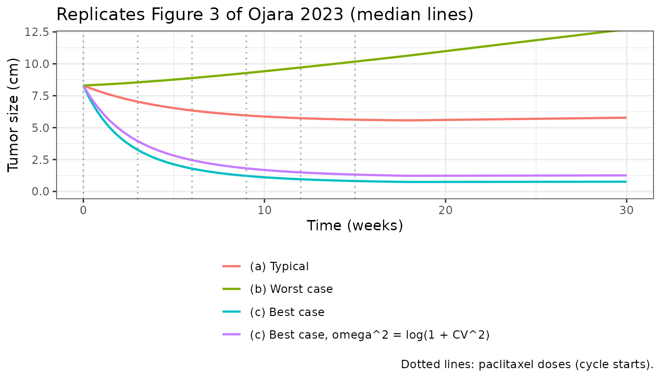
Values read off Figure 3 of the paper are compared with the simulation below.
fig3_paper <- tibble::tribble(
  ~scenario, ~week, ~paper_cm,
  "(a) Typical", 6, 6.3,
  "(a) Typical", 12, 5.7,
  "(a) Typical", 18, 5.5,
  "(a) Typical", 30, 5.5,
  "(c) Best case", 6, 1.8,
  "(c) Best case", 18, 0.75,
  "(c) Best case", 30, 0.7
)
fig3_cmp <- fig3_paper |>
  left_join(
    sim_fig3 |>
      mutate(week = time / 168) |>
      select(scenario, week, model_cm = tumor_size) |>
      mutate(model_cm = model_cm / 10),
    by = c("scenario", "week")
  )
fig3_logcv <- sim_fig3 |>
  filter(scenario == "(c) Best case, omega^2 = log(1 + CV^2)", time %in% (c(6, 18, 30) * 168)) |>
  pull(tumor_size) / 10
fig3_cmp$model_logcv_cm <- c(rep(NA, 4), fig3_logcv)
fig3_cmp |>
  dplyr::rename(
    Scenario = scenario, Week = week, "Figure 3 (cm)" = paper_cm,
    "Model (cm)" = model_cm, "Model, omega^2 = log(1 + CV^2) (cm)" = model_logcv_cm
  ) |>
knitr::kable(digits = 2)| Scenario | Week | Figure 3 (cm) | Model (cm) | Model, omega^2 = log(1 + CV^2) (cm) |
|---|---|---|---|---|
| (a) Typical | 6 | 6.30 | 6.34 | NA |
| (a) Typical | 12 | 5.70 | 5.74 | NA |
| (a) Typical | 18 | 5.50 | 5.57 | NA |
| (a) Typical | 30 | 5.50 | 5.78 | NA |
| (c) Best case | 6 | 1.80 | 1.79 | 2.45 |
| (c) Best case | 18 | 0.75 | 0.74 | 1.23 |
| (c) Best case | 30 | 0.70 | 0.76 | 1.26 |
typ <- fig3_cmp$scenario == "(a) Typical"
best <- fig3_cmp$scenario == "(c) Best case"
stopifnot(
  abs(fig3_cmp$model_cm[typ] / fig3_cmp$paper_cm[typ] - 1) < 0.1,
  # Values read off a figure: 15% admits the reading error, while the
  # alternative omega scale is 35-80% off at every time point.
  abs(fig3_cmp$model_cm[best] / fig3_cmp$paper_cm[best] - 1) < 0.15,
  all(fig3_cmp$model_logcv_cm[best] / fig3_cmp$paper_cm[best] > 1.3)
)
The typical profile (panel a) matches the figure within a few
percent. This also settles a units question: the Results text says a
threshold AUCcycle of 4.49 umolh/L is needed to start shrinkage,
which equals Kg / beta02_pac without the tumor size factor
that Equation 2 requires. With the tumor size included the threshold is
Kg / (beta02_pac * 83 mm) = 0.54 umolh/L. A Kg
8.3-fold larger, which would make the 4.49 statement exact, would have
the typical tumor regrowing to about 9 cm by week 30, which Figure 3a
does not show. The Table 1 value is used.
Panel (c) discriminates between the two usual readings of the CV%
that Table 1 reports for the exponential IIV model. With
omega^2 = (CV/100)^2 the best case plateaus near 0.75 cm,
as in Figure 3c; with omega^2 = log(1 + CV^2) it plateaus
near 1.2 cm. The model uses (CV/100)^2. The worst-case
panel (b), which shows a nadir near 7.4 cm at week 8 before regrowth to
about 9 cm, is not reproduced by either reading (both give a monotonic
increase): with Kg at its 97.5th percentile it implies a decay rate only
about 1.6-fold below the typical value. The paper does not say how the
percentiles of panel (b) were obtained.
Virtual cohort: week-8 tumor size and dropout
The paper does not report the distribution of AUCcycle beyond its median and range. The cohort below draws one AUCcycle per subject from a log-normal distribution with median 18.4 umol*h/L and log-scale SD 0.3, truncated to the published range 3.82-33.3, and keeps it for all six cycles. Baseline tumor size is log-normal with median 83 mm and log-scale SD 0.6, truncated to the published range 10-383 mm (Table S1). These distributions are assumptions of this vignette.
set.seed(20231101)
rxode2::rxSetSeed(20231101)
n_sub <- 200
cohort <- tibble::tibble(
  id = seq_len(n_sub),
  auc = pmin(pmax(18.4 * exp(rnorm(n_sub, 0, 0.3)), 3.82), 33.3),
  base_mm = pmin(pmax(83 * exp(rnorm(n_sub, 0, 0.6)), 10), 383)
)
week8_h <- 8 * 168
obs_cohort <- sort(unique(c(seq(0, 30 * 168, by = 168), end_tx_h, week8_h)))
ev_cohort <- cohort |>
  tidyr::expand_grid(time = obs_cohort) |>
  mutate(
    evid = 0, amt = 0, cmt = "tumor_size",
    TUMSZ = base_mm,
    AUC_PTX = ifelse(time < end_tx_h, auc, 0)
  ) |>
  select(id, time, evid, amt, cmt, TUMSZ, AUC_PTX)

sim_cohort <- rxode2::rxSolve(
  tgi, events = ev_cohort, covsInterpolation = "locf",
  returnType = "data.frame"
)
#> ℹ parameter labels from comments will be replaced by 'label()'
sim_cohort |>
  group_by(time) |>
  summarise(
    p05 = quantile(sim / TUMSZ, 0.05),
    p50 = quantile(sim / TUMSZ, 0.50),
    p95 = quantile(sim / TUMSZ, 0.95),
    .groups = "drop"
  ) |>
  ggplot(aes(time / 168)) +
  geom_ribbon(aes(ymin = 100 * p05, ymax = 100 * p95), alpha = 0.25) +
  geom_line(aes(y = 100 * p50)) +
  labs(
    x = "Time (weeks)", y = "Tumor size (% of baseline)",
    title = "Simulated tumor size relative to baseline (median, 5th-95th percentiles)",
    caption = "Compare with Figure 1 of Ojara 2023 (observed data, no dropout applied here)."
  ) +
  theme_bw()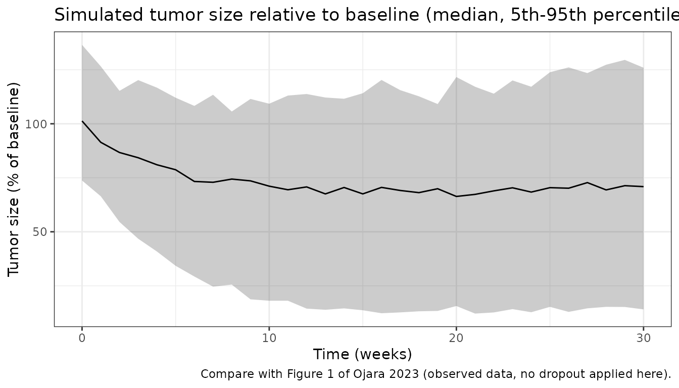
The paper reports a median model-derived RS8 of 80% (a 20.0% reduction, range -78% to +15%) across the individual (empirical Bayes) predictions. The simulated week-8 values below use the individual model predictions without residual error.
rs8 <- sim_cohort |>
  filter(time == week8_h) |>
  transmute(id, RCFB8_SLD = tumor_size / TUMSZ - 1)
rs8_summary <- tibble::tibble(
  Statistic = c("Median RS8 (%)", "5th percentile RS8 (%)", "95th percentile RS8 (%)"),
  Simulated = 100 * (1 + quantile(rs8$RCFB8_SLD, c(0.5, 0.05, 0.95), names = FALSE)),
  Paper = c(80.0, 42.4, 91.4)
)
knitr::kable(rs8_summary, digits = 1)| Statistic | Simulated | Paper |
|---|---|---|
| Median RS8 (%) | 75.2 | 80.0 |
| 5th percentile RS8 (%) | 21.9 | 42.4 |
| 95th percentile RS8 (%) | 97.2 | 91.4 |
The paper’s 5th and 95th RS8 percentiles (Table S5) come from the shrunken individual estimates of the 221-patient subset, so the simulated spread, which samples the full IIV, is wider.
The dropout model integrates the hazard
lambda0 * exp(-1.88 * shrinkage). At no change in tumor
size the hazard is 4.7 per 10,000 patients per hour and at a 10%
shrinkage 3.9, the “5 versus 4 in 10,000” quoted in Appendix S1. Of the
365 patients, 84 (23%) still had tumor assessments after week 30
(Results).
haz <- exp(th[["llam_haz"]]) * exp(th[["e_tsshrink_haz"]] * c(0, 0.1)) * 1e4
knitr::kable(
  tibble::tibble(
    "Relative shrinkage" = c(0, 0.1),
    "Hazard per 10,000 patients per hour" = haz
  ),
  digits = 2
)| Relative shrinkage | Hazard per 10,000 patients per hour |
|---|---|
| 0.0 | 4.73 |
| 0.1 | 3.92 |
stopifnot(round(haz) == c(5, 4))

stay30 <- sim_cohort |>
  filter(time == 30 * 168) |>
  summarise(stay = mean(sur_drop)) |>
  pull(stay)
stay30
#> [1] 0.2550799
stopifnot(stay30 > 0.15, stay30 < 0.35)
The simulated probability of remaining in tumor follow-up at week 30 is 26%, against 23% observed.
Overall survival model
Closed-form checks
With no interindividual variability, the Weibull survival function is
S(t) = exp(-(lambda * t)^alpha * exp(E_CRP * (CRP - 23.5)) * exp(E_RS8 * (RS8 - 80))).
The paper quotes a median OS of 45 weeks at the median covariates, 103
weeks when both covariates are at their 5th percentiles (CRP 1.18 mg/L,
RS8 42.4%) and 18.2 weeks when both are at their 95th percentiles (151
mg/L, 91.4%).
ini_os <- os()$iniDf
tho <- setNames(ini_os$est, ini_os$name)
median_os_wk <- function(crp, rs8_pct) {
  m <- exp(tho[["e_crp_haz"]] * (crp - 23.5) + tho[["e_rcfb8_haz"]] * (rs8_pct - 80))
  (log(2) / m)^(1 / exp(tho[["lalfa_haz"]])) / exp(tho[["llam_haz"]]) / 168
}
os_checks <- tibble::tibble(
  Covariates = c("Medians (CRP 23.5, RS8 80%)", "Both 5th percentiles", "Both 95th percentiles"),
  CRP = c(23.5, 1.18, 151),
  RS8 = c(80, 42.4, 91.4),
  Paper = c(45, 103, 18.2)
) |>
  mutate(Model = median_os_wk(CRP, RS8))
os_checks |>
  dplyr::rename("CRP (mg/L)" = CRP, "RS8 (%)" = RS8, "Paper median OS (weeks)" = Paper, "Model median OS (weeks)" = Model) |>
knitr::kable(digits = 1)| Covariates | CRP (mg/L) | RS8 (%) | Paper median OS (weeks) | Model median OS (weeks) |
|---|---|---|---|---|
| Medians (CRP 23.5, RS8 80%) | 23.5 | 80.0 | 45.0 | 44.8 |
| Both 5th percentiles | 1.2 | 42.4 | 103.0 | 100.5 |
| Both 95th percentiles | 151.0 | 91.4 | 18.2 | 17.5 |
The same medians follow from solving the packaged model (the
cumulative hazard is integrated as an ODE, as in the NONMEM
$DES block):
ev_os <- tidyr::expand_grid(
  tibble::tibble(id = 1:3, CRP = os_checks$CRP, RCFB8_SLD = os_checks$RS8 / 100 - 1),
  time = seq(0, 200 * 168, by = 24)
) |>
  mutate(evid = 0, amt = 0, cmt = "cumhaz")
sim_os <- rxode2::rxSolve(os, events = ev_os, returnType = "data.frame")
solved_median <- sim_os |>
  group_by(id) |>
  summarise(median_wk = approx(sur, time, 0.5)$y / 168, .groups = "drop")
knitr::kable(solved_median, digits = 1)| id | median_wk |
|---|---|
| 1 | 44.8 |
| 2 | 100.5 |
| 3 | 17.5 |
Table S5 and Figure 5: one covariate at a time
Table S5 varies one covariate across its percentiles while the other follows its distribution in the CEPAC-TDM data, and reports the median of the simulated Kaplan-Meier curve. The individual data are not available, so the other covariate is taken here as 200 equally spaced quantiles of a distribution interpolated (on the log scale for CRP) through the published percentiles: CRP 0.34 / 1.18 / 8.07 / 23.5 / 55.3 / 151 / 281 mg/L at the 0 / 5 / 25 / 50 / 75 / 95 / 100th percentiles (Tables S2 and S5) and RS8 22 / 42.4 / 64.8 / 80.0 / 86.0 / 91.4 / 115% (Results range and Table S5). CRP and RS8 are treated as independent.
qgrid <- (seq_len(200) - 0.5) / 200
p_known <- c(0, 0.05, 0.25, 0.5, 0.75, 0.95, 1)
crp_q <- exp(approx(p_known, log(c(0.34, 1.18, 8.07, 23.5, 55.3, 151, 281)), qgrid)$y)
rs8_q <- approx(p_known, c(22, 42.4, 64.8, 80.0, 86.0, 91.4, 115), qgrid)$y

tabS5 <- tibble::tribble(
  ~covariate, ~level, ~paper_wk,
  "RS8", 42.4, 82.3,
  "RS8", 64.8, 57.4,
  "RS8", 86.0, 41.8,
  "RS8", 91.4, 34.0,
  "CRP", 1.18, 56.7,
  "CRP", 8.07, 51.0,
  "CRP", 55.3, 38.8,
  "CRP", 151.0, 24.0
) |>
  mutate(arm = seq_len(n()))

ev_s5 <- tabS5 |>
  tidyr::expand_grid(k = seq_along(qgrid)) |>
  mutate(
    id = (arm - 1) * length(qgrid) + k,
    CRP = ifelse(covariate == "CRP", level, crp_q[k]),
    RCFB8_SLD = ifelse(covariate == "RS8", level, rs8_q[k]) / 100 - 1
  ) |>
  select(id, arm, CRP, RCFB8_SLD) |>
  tidyr::expand_grid(time = seq(0, 200 * 168, by = 84)) |>
  mutate(evid = 0, amt = 0, cmt = "cumhaz")

sim_s5 <- rxode2::rxSolve(os, events = ev_s5, keep = "arm", returnType = "data.frame")
pop_surv <- sim_s5 |>
  group_by(arm, time) |>
  summarise(sur = mean(sur), .groups = "drop")
s5_cmp <- pop_surv |>
  group_by(arm) |>
  summarise(model_wk = approx(sur, time, 0.5)$y / 168, .groups = "drop") |>
  right_join(tabS5, by = "arm")
s5_cmp |>
  select(covariate, level, paper_wk, model_wk) |>
  dplyr::rename(
    Covariate = covariate, "Level (CRP mg/L or RS8 %)" = level,
    "Table S5 median OS (weeks)" = paper_wk, "Model median OS (weeks)" = model_wk
  ) |>
knitr::kable(digits = 1)| Covariate | Level (CRP mg/L or RS8 %) | Table S5 median OS (weeks) | Model median OS (weeks) |
|---|---|---|---|
| RS8 | 42.4 | 82.3 | 78.6 |
| RS8 | 64.8 | 57.4 | 52.4 |
| RS8 | 86.0 | 41.8 | 35.8 |
| RS8 | 91.4 | 34.0 | 32.4 |
| CRP | 1.2 | 56.7 | 55.6 |
| CRP | 8.1 | 51.0 | 53.4 |
| CRP | 55.3 | 38.8 | 40.7 |
| CRP | 151.0 | 24.0 | 23.4 |
stopifnot(
  abs(median(s5_cmp$model_wk / s5_cmp$paper_wk - 1)) < 0.1,
  max(abs(s5_cmp$model_wk / s5_cmp$paper_wk - 1)) < 0.2
)
pop_surv |>
  left_join(tabS5, by = "arm") |>
  filter(level %in% c(42.4, 91.4, 1.18, 151)) |>
  mutate(
    panel = ifelse(covariate == "CRP", "(a) Baseline CRP", "(b) RS8"),
    percentile = ifelse(level %in% c(42.4, 1.18), "5th percentile", "95th percentile")
  ) |>
  ggplot(aes(time / 168, sur, linetype = percentile)) +
  geom_line() +
  facet_wrap(~panel) +
  coord_cartesian(xlim = c(0, 150)) +
  labs(
    x = "Time (weeks)", y = "Probability of survival", linetype = NULL,
    title = "Replicates Figure 5 of Ojara 2023 (median curves)"
  ) +
  theme_bw() +
  theme(legend.position = "bottom")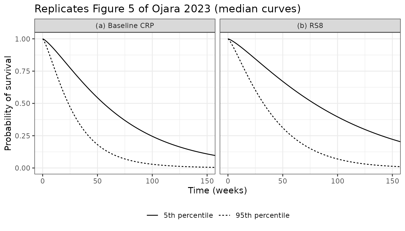
Linking the two models
In the paper the OS model receives RS8 from the TGI model. The chunk below feeds the week-8 tumor sizes of the simulated TGI cohort into the OS model, pairing them with CRP values drawn from the interpolated CRP distribution.
linked <- rs8 |>
  mutate(CRP = sample(crp_q, n(), replace = TRUE)) |>
  tidyr::expand_grid(time = seq(0, 200 * 168, by = 84)) |>
  mutate(evid = 0, amt = 0, cmt = "cumhaz")
sim_linked <- rxode2::rxSolve(os, events = linked, returnType = "data.frame")
linked_median <- sim_linked |>
  group_by(time) |>
  summarise(sur = mean(sur), .groups = "drop") |>
  summarise(median_wk = approx(sur, time, 0.5)$y / 168) |>
  pull(median_wk)
linked_median
#> [1] 46.32316
The population median OS of the linked simulation is 46.3 weeks, against an observed median of 11.3 months (about 49 weeks) in the abstract and a typical model value of 45 weeks.
PKNCA
The packaged models take paclitaxel exposure as an input (AUCcycle) and have no drug concentration output, so there is no concentration-time profile on which to run a non-compartmental analysis. The checks above are on the quantities the paper reports for these models.
Assumptions and deviations
-
IIV scale. Table 1 reports IIV as CV% without
stating the formula. The variances are
(CV/100)^2, the reading that reproduces the best-case profile of Figure 3c (see above). Underlog(1 + CV^2)the variances would be 0.862, 0.557 and 0.254 instead of 1.369, 0.745 and 0.291. The residual error CV of 17.9% is used as the log-scale SD in the same way. - Kg units. Kg is 1.03 um/h in Table 1 and is stored as 1.03e-3 mm/h. The Results statement that an AUCcycle of 4.49 umol*h/L is needed to start tumor shrinkage omits the tumor size from Equation 2; the Table 1 value is confirmed by Figure 3a and by the Discussion’s 0.587 cm/week.
- Paclitaxel exposure as an input. The TGI model is driven by AUCcycle, which the authors derived from the paclitaxel PK model of Henrich et al. (2017, J Pharmacol Exp Ther 362:347-358). That PK model is not part of this package, so the user supplies AUC_PTX directly as a step covariate that is constant within each 21-day cycle and 0 after the last cycle ends. The paper defines AUCcycle per cycle but does not state the value after treatment ends; 0 is used, since no paclitaxel is given then.
-
Time origin. The drug-effect decline
exp(-res * t)uses the model time, so time 0 must be the first paclitaxel dose. - Platinum drugs. Carboplatin and cisplatin were given at the same time as paclitaxel; their effect could not be separated and is absorbed into the paclitaxel drug effect, as in the paper.
- Dropout model. The dropout model of Table S4 (right column, both arms) is included in the TGI file because it depends on the predicted tumor size. Its reference BASE is taken as the observed baseline tumor size (TUMSZ).
-
RS8 covariate. The paper’s RS8 (percent of
baseline) enters the OS model as
RCFB8_SLD, the fractional change from baseline, withRS8 = 100 * (1 + RCFB8_SLD)computed insidemodel(); the coefficient and the centring value of 80.0% are unchanged. - Virtual cohorts. The AUCcycle and baseline tumor size distributions of the TGI cohort, and the CRP and RS8 distributions used for Table S5, are interpolations of the published medians, percentiles and ranges, not the trial data. CRP and RS8 are treated as independent.
-
Sex percentage.
population$sex_female_pctof the TGI file is from the 221-patient subset (Table S1); the paper does not tabulate demographics of all 365 patients.