Vancomycin (Parasuraman 2021) • nlmixr2lib

Model and source

mod <- readModelDb("Parasuraman_2021_vancomycin")
mod_ui <- rxode2::rxode2(mod)
#> ℹ parameter labels from comments will be replaced by 'label()'

Citation: Parasuraman JM, Kloprogge F, Standing JF, Albur M, Heep A. Population pharmacokinetics of intraventricular vancomycin in neonatal ventriculitis, a preterm pilot study. Eur J Pharm Sci. 2021;158:105643. doi:10.1016/j.ejps.2020.105643. Size and maturation form from Germovsek E, Barker CIS, Sharland M, Standing JF. Scaling clearance in paediatric pharmacokinetics: all models are wrong, which are useful? Br J Clin Pharmacol. 2017;83(4):777-790. doi:10.1111/bcp.13160 (Table 1, model 9b).
Description: Parallel one-compartment plasma and one-compartment CSF population PK model for intravenous and intraventricular vancomycin in extremely preterm infants (<28 weeks gestation) treated for ventriculitis (Parasuraman 2021). Plasma CL and V are allometrically scaled to 70 kg (fixed exponents 0.632 on CL, 1 on V) with a fixed Rhodin postmenstrual-age maturation sigmoid on CL; the CSF compartment receives intraventricular doses and has its own clearance and volume, with no plasma-CSF transfer.
Article: https://doi.org/10.1016/j.ejps.2020.105643 (open access, PMC7848885)
Size and maturation framework: Germovsek et al. 2017, https://doi.org/10.1111/bcp.13160 (Table 1, model 9b)

Parasuraman et al. pooled intravenous (IV) and intraventricular vancomycin data from eight extremely preterm infants treated for ventriculitis through a ventricular access device (Ommaya reservoir). The final model is two parallel, unconnected one-compartment models: plasma (IV doses) and CSF (intraventricular doses). Transfer between plasma and CSF in either direction did not improve the fit, so the published model has none. Ventricular index, CSF protein and serum creatinine were all tested and none was retained.

Population

Eight preterm infants born at <28 weeks gestation (median gestational age 25.3 weeks, range 23.9-27.7; median birth weight 0.78 kg, range 0.517-1.13 kg; 62.5% female) were treated for ventriculitis at Southmead Hospital NICU, Bristol, UK, between 2009 and 2016 (Table 2). At the time of treatment the median postnatal age was 8.7 weeks (3.9-23.1) and the median postmenstrual age 34.4 weeks (30.2-48.1). Intraventricular starting doses were 3, 5, 10 or 15 mg, given as a 2-minute slow bolus of a 10 mg/mL solution, and were repeated when the CSF level fell below 10 mg/L. Six of the eight infants also received IV vancomycin at 15 mg/kg every 24 h (<29 weeks PMA) or every 12 h (29-35 weeks PMA). The final analysis used 37 plasma concentrations from 5 infants and 67 CSF concentrations from 8 infants.

The same information is available programmatically:

str(mod_ui$population)
#> List of 16
#>  $ species              : chr "human"
#>  $ n_subjects           : int 8
#>  $ n_studies            : int 1
#>  $ age_range            : chr "Postnatal age 3.9-23.1 weeks; postmenstrual age 30.2-48.1 weeks"
#>  $ age_median           : chr "Postnatal age 8.7 weeks; postmenstrual age 34.4 weeks"
#>  $ gestational_age_range: chr "23.9-27.7 weeks (median 25.3)"
#>  $ weight_range         : chr "Birth weight 0.517-1.13 kg (current weight at sampling not reported)"
#>  $ weight_median        : chr "Birth weight 0.78 kg"
#>  $ sex_female_pct       : num 62.5
#>  $ race_ethnicity       : chr "Not reported"
#>  $ disease_state        : chr "Extremely preterm infants (<28 weeks gestation) with ventriculitis (CSF white cell count >20/mm^3 or positive C"| __truncated__
#>  $ dose_range           : chr "Intraventricular vancomycin starting doses of 3, 5, 10 or 15 mg (10 mg/mL slow bolus over 2 min via the reservo"| __truncated__
#>  $ regions              : chr "United Kingdom (Southmead Hospital NICU, Bristol), 2009-2016"
#>  $ samples_plasma       : chr "37 plasma concentrations from 5 infants (median 5 per infant, range 2-18)"
#>  $ samples_csf          : chr "67 CSF concentrations from 8 infants (median 7.5 per infant, range 4-16)"
#>  $ notes                : chr "Retrospective single-centre case review; demographics from Table 2. CSF drainage was fairly constant at 5-10 mL"| __truncated__

Source trace

Every ini() value carries an in-file source comment in inst/modeldb/specificDrugs/Parasuraman_2021_vancomycin.R; the table collects them.

Parameter / equation	Value	Source location
`lcl` (plasma CL per 70 kg, fully mature)	log(9.29) L/h	Table 3, CL = 9.29 L/h/70 kg
`lvc` (plasma V per 70 kg)	log(54.4) L	Table 3, V = 54.4 L/70 kg
`lcl_csf` (CSF clearance)	log(0.002) L/h	Table 3, CLCSF = 0.002 L/h
`lvcsf` (CSF volume)	log(0.109) L	Table 3, VCSF = 0.109 L
`e_wt_cl`	0.632 (fixed)	Methods ‘NLME modelling’: weight standardised to 70 kg, allometric exponent 0.632
`e_wt_vc`	1 (fixed)	Table 3 reports V per 70 kg (linear scaling)
`tmat50`	55.4 weeks (fixed)	Not printed; Germovsek 2017 Table 1 model 9b (the 0.632-exponent pairing), cited by the paper for its a priori size-and-age scaling
`hill`	3.33 (fixed)	As `tmat50`
`etalcl`	0.0676	Table 3, IIV CL 26% CV; footnote CV = 100 x omega
`etalcl_csf`	0.0841	Table 3, IIV CLCSF 29% CV
`etalvcsf`	0.36	Table 3, IIV VCSF 60% CV
IIV on V	none	Table 3, 0 FIX
`propSd`	0.3131	Table 3, sigma prop plasma 31.31% CV
`propSd_Ccsf`	0.458	Table 3, sigma prop CSF 45.8% CV
`d/dt(central) <- -cl/vc * central`	n/a	Methods, dA(p)/dt equation
`d/dt(csf) <- -cl_csf/vcsf * csf`	n/a	Methods, dA(csf)/dt equation
`fmat <- PAGE^hill / (tmat50^hill + PAGE^hill)`	n/a	Methods (“maturation function”, citing Germovsek 2016 and 2017); form from Germovsek 2017 Table 1 model 9b

Virtual cohort

The paper reports birth weight but not the weight at the time of treatment, which is what the allometric model needs. The cohort below draws postmenstrual age from the published range and assigns a current weight from a simple linear growth assumption (1.6 kg at the median 34.4 weeks PMA, +0.18 kg per week, with 12% log-normal scatter). Both are assumptions by the maintainers; see Assumptions and deviations.

Every virtual infant receives one 10 mg intraventricular dose at time 0 into csf, and 15 mg/kg IV vancomycin as a 1-hour infusion every 12 hours for ten doses into central. Because the two compartments are not connected, the two routes can share one event table without influencing each other.

set.seed(20210107)
rxode2::rxSetSeed(20210107)
n_sub <- 200L

# Postmenstrual age: reject-and-redraw inside the published range
# (Table 2: 30.2-48.1 weeks, median 34.4).
draw_pma <- function(n) {
  out <- numeric(0)
  while (length(out) < n) {
    x <- exp(rnorm(n, log(34.4), 0.12))
    out <- c(out, x[x >= 30.2 & x <= 48.1])
  }
  out[seq_len(n)]
}

cohort <- tibble(
  id = seq_len(n_sub),
  PAGE = draw_pma(n_sub)
) |>
  mutate(WT = pmax(0.6, 1.6 + 0.18 * (PAGE - 34.4)) * exp(rnorm(n_sub, 0, 0.12)))

iv_times <- seq(0, 108, by = 12)
obs_times <- sort(unique(c(seq(0, 72, by = 0.25), seq(108, 120, by = 0.1))))

build_events <- function(cohort, ivt_dose = 10) {
  ivt <- cohort |>
    mutate(time = 0, amt = ivt_dose, rate = 0, evid = 1L, cmt = "csf")
  iv <- cohort |>
    tidyr::crossing(time = iv_times) |>
    mutate(amt = 15 * WT, rate = amt / 1, evid = 1L, cmt = "central")
  obs <- cohort |>
    tidyr::crossing(time = obs_times) |>
    mutate(amt = 0, rate = 0, evid = 0L, cmt = "central")
  # Two endpoints (Cc, Ccsf): observation rows sit on an ODE state and carry
  # dvid = 1 so rxode2 can map them; rxode2 returns BOTH Cc and Ccsf on every
  # observation row, so one observation grid serves both matrices.
  bind_rows(ivt, iv, obs) |>
    mutate(dvid = ifelse(evid == 0L, 1L, NA_integer_)) |>
    arrange(id, time, desc(evid)) |>
    as.data.frame()
}
events <- build_events(cohort)
stopifnot(!anyDuplicated(unique(events[, c("id", "time", "evid", "cmt")])))

Simulation

sim <- rxode2::rxSolve(
  mod,
  events = events,
  keep = c("WT", "PAGE"),
  returnType = "data.frame"
)
#> ℹ parameter labels from comments will be replaced by 'label()'

# Residual error added in R so the VPC below matches the paper's
# observation-level percentiles (proportional on each matrix).
th <- rxode2::rxode2(mod)$theta
#> ℹ parameter labels from comments will be replaced by 'label()'
sim <- sim |>
  mutate(
    Cc_obs = Cc * (1 + th[["propSd"]] * rnorm(n())),
    Ccsf_obs = Ccsf * (1 + th[["propSd_Ccsf"]] * rnorm(n()))
  )

Closed-form checks (typical values)

With the random effects set to zero, the CSF compartment after an intraventricular bolus is a mono-exponential with C0 = dose / vcsf and k = cl_csf / vcsf, and the plasma profile after ten 1-hour infusions is the superposition of ten one-compartment infusion curves. Both are recomputed analytically from the ini() values and compared with the solver.

mod_typ <- rxode2::zeroRe(mod)
#> ℹ parameter labels from comments will be replaced by 'label()'
typ_cov <- data.frame(id = 1L, WT = 1.6, PAGE = 34.4)
ev_typ <- build_events(typ_cov)
sim_typ <- rxode2::rxSolve(
  mod_typ,
  events = ev_typ,
  returnType = "data.frame",
  atol = 1e-10, rtol = 1e-10
)
#> ℹ omega/sigma items treated as zero: 'etalcl', 'etalcl_csf', 'etalvcsf'

cl_typ <- exp(th[["lcl"]]) * (1.6 / 70)^th[["e_wt_cl"]] *
  34.4^th[["hill"]] / (th[["tmat50"]]^th[["hill"]] + 34.4^th[["hill"]])
v_typ <- exp(th[["lvc"]]) * (1.6 / 70)^th[["e_wt_vc"]]
k_typ <- cl_typ / v_typ
vcsf_typ <- exp(th[["lvcsf"]])
kcsf_typ <- exp(th[["lcl_csf"]]) / vcsf_typ

csf_analytic <- 10 / vcsf_typ * exp(-kcsf_typ * sim_typ$time)
inf_one <- function(t, t0, dose, tinf = 1) {
  r <- dose / tinf
  tt <- t - t0
  ifelse(
    tt <= 0, 0,
    ifelse(
      tt <= tinf,
      r / cl_typ * (1 - exp(-k_typ * tt)),
      r / cl_typ * (1 - exp(-k_typ * tinf)) * exp(-k_typ * (tt - tinf))
    )
  )
}
cc_analytic <- Reduce(`+`, lapply(iv_times, function(t0) inf_one(sim_typ$time, t0, 15 * 1.6)))

rel_csf <- abs(sim_typ$Ccsf - csf_analytic) / csf_analytic
rel_cc <- abs(sim_typ$Cc - cc_analytic)[sim_typ$time > 0] / cc_analytic[sim_typ$time > 0]
c(max_rel_err_csf = max(rel_csf), max_rel_err_plasma = max(rel_cc))
#>    max_rel_err_csf max_rel_err_plasma 
#>       1.836388e-11       2.326819e-10
stopifnot(max(rel_csf) < 1e-5, max(rel_cc) < 1e-5)

typical <- tibble(
  quantity = c(
    "Plasma CL (L/h), 1.6 kg, 34.4 wk PMA", "Plasma V (L)", "Plasma t1/2 (h)",
    "CSF CL (L/h)", "CSF V (L)", "CSF t1/2 (h)",
    "CSF C0 after 10 mg (mg/L)", "Time for CSF to fall to 10 mg/L after 10 mg (h)"
  ),
  value = c(
    cl_typ, v_typ, log(2) / k_typ,
    exp(th[["lcl_csf"]]), vcsf_typ, log(2) / kcsf_typ,
    10 / vcsf_typ, log(10 / vcsf_typ / 10) / kcsf_typ
  )
)
knitr::kable(typical, digits = 3, caption = "Typical-value quantities implied by Table 3.")

Typical-value quantities implied by Table 3.
quantity	value
Plasma CL (L/h), 1.6 kg, 34.4 wk PMA	0.145
Plasma V (L)	1.243
Plasma t1/2 (h)	5.950
CSF CL (L/h)	0.002
CSF V (L)	0.109
CSF t1/2 (h)	37.777
CSF C0 after 10 mg (mg/L)	91.743
Time for CSF to fall to 10 mg/L after 10 mg (h)	120.794

The typical CSF half-life is about 38 h, so a 10 mg dose stays above the 10 mg/L re-dosing threshold for roughly five days in a typical infant.

Replicate published figures

Figure 2: VPC versus time after dose

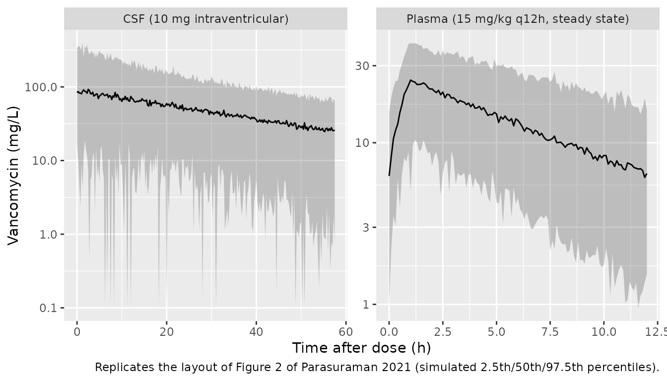
Figure 2 of the paper is a prediction-corrected VPC of plasma (left) and CSF (right) concentrations against time after dose. The observed data are not available, so the panels below show the simulated 2.5th, 50th and 97.5th percentiles for the virtual cohort (plasma: last dosing interval at steady state; CSF: after a single 10 mg intraventricular dose over the observed 0-57 h time-after-dose range).

vpc <- bind_rows(
  sim |>
    filter(time >= 108, time <= 120) |>
    transmute(id, tad = time - 108, conc = Cc_obs, matrix = "Plasma (15 mg/kg q12h, steady state)"),
  sim |>
    filter(time <= 57.5) |>
    transmute(id, tad = time, conc = Ccsf_obs, matrix = "CSF (10 mg intraventricular)")
) |>
  group_by(matrix, tad) |>
  summarise(
    p025 = quantile(conc, 0.025),
    p50 = quantile(conc, 0.5),
    p975 = quantile(conc, 0.975),
    .groups = "drop"
  )

ggplot(vpc, aes(tad, p50)) +
  geom_ribbon(aes(ymin = pmax(p025, 0.1), ymax = p975), alpha = 0.25) +
  geom_line() +
  facet_wrap(~matrix, scales = "free") +
  scale_y_log10() +
  labs(
    x = "Time after dose (h)", y = "Vancomycin (mg/L)",
    caption = "Replicates the layout of Figure 2 of Parasuraman 2021 (simulated 2.5th/50th/97.5th percentiles)."
  )

Comparison with the observed concentration ranges (Table 2)

Table 2 reports observed plasma concentrations of median 8.6 mg/L (range 2.2-26.6) at a median 5.59 h after dose, and CSF concentrations of median 24.9 mg/L (range 2.5-230.7) at a median 7.39 h after dose. The observed CSF data pool starting doses of 3 to 15 mg and repeat doses, so the single 10 mg scenario is expected to sit toward the upper part of the CSF range rather than on its median. Likewise, routine plasma monitoring was a pre-dose level before the third and later IV doses (Methods), so the observed plasma median leans toward troughs, whereas the simulated summary spans the whole dosing interval; the simulated steady-state Cmin in the PKNCA section below is the closer comparator.

obs_cmp <- bind_rows(
  sim |>
    filter(time >= 108, time <= 122) |>
    summarise(
      simulated_median = median(Cc_obs),
      simulated_p05 = quantile(Cc_obs, 0.05),
      simulated_p95 = quantile(Cc_obs, 0.95)
    ) |>
    mutate(matrix = "Plasma, steady-state interval", observed = "8.6 (2.2-26.6)"),
  sim |>
    filter(time <= 57.5) |>
    summarise(
      simulated_median = median(Ccsf_obs),
      simulated_p05 = quantile(Ccsf_obs, 0.05),
      simulated_p95 = quantile(Ccsf_obs, 0.95)
    ) |>
    mutate(matrix = "CSF, 0-57 h after 10 mg", observed = "24.9 (2.5-230.7)")
) |>
  relocate(matrix, observed)

obs_cmp |>
  rename(
    "Matrix" = matrix,
    "Observed median (range), Table 2" = observed,
    "Simulated median" = simulated_median,
    "Simulated 5th pct" = simulated_p05,
    "Simulated 95th pct" = simulated_p95
  ) |>
  knitr::kable(digits = 1, caption = "Simulated concentrations (mg/L) versus the observed ranges in Table 2.")

Simulated concentrations (mg/L) versus the observed ranges in Table 2.
Matrix	Observed median (range), Table 2	Simulated median	Simulated 5th pct	Simulated 95th pct
Plasma, steady-state interval	8.6 (2.2-26.6)	12.6	3.5	28.9
CSF, 0-57 h after 10 mg	24.9 (2.5-230.7)	44.6	7.9	149.8


# Unit / scale guard: a volume entered in mL instead of L, or a per-kg value
# read as per-70-kg, moves these medians by orders of magnitude.
stopifnot(
  obs_cmp$simulated_median[1] > 2.2, obs_cmp$simulated_median[1] < 26.6,
  obs_cmp$simulated_median[2] > 2.5, obs_cmp$simulated_median[2] < 230.7
)

PKNCA validation

CSF: single intraventricular dose by starting dose

The paper’s four intraventricular starting doses (3, 5, 10, 15 mg) are simulated with typical parameters and analysed with PKNCA. The paper reports no NCA table, so the reference values are the analytic single-dose values implied by Table 3 (Cmax = dose / VCSF, AUCinf = dose / CLCSF, t1/2 = ln 2 * VCSF / CLCSF).

ivt_doses <- c(3, 5, 10, 15)
ev_csf <- bind_rows(lapply(seq_along(ivt_doses), function(i) {
  d <- ivt_doses[i]
  bind_rows(
    data.frame(id = i, time = 0, amt = d, evid = 1L, cmt = "csf"),
    data.frame(id = i, time = c(0, seq(0.25, 2, 0.25), seq(3, 336, 1)), amt = 0, evid = 0L, cmt = "csf")
  ) |>
    mutate(
      WT = 1.6, PAGE = 34.4, treatment = paste(d, "mg"),
      dvid = ifelse(evid == 0L, 2L, NA_integer_)
    )
}))

sim_csf <- rxode2::rxSolve(mod_typ, events = ev_csf, keep = "treatment", returnType = "data.frame")
#> ℹ omega/sigma items treated as zero: 'etalcl', 'etalcl_csf', 'etalvcsf'
#> Warning: multi-subject simulation without without 'omega'

conc_csf <- sim_csf |>
  filter(!is.na(Ccsf)) |>
  select(id, time, Ccsf, treatment)
dose_csf <- ev_csf |>
  filter(evid == 1) |>
  select(id, time, amt, treatment)

nca_csf <- PKNCA::pk.nca(PKNCA::PKNCAdata(
  PKNCA::PKNCAconc(conc_csf, Ccsf ~ time | treatment + id, concu = "mg/L", timeu = "h"),
  PKNCA::PKNCAdose(dose_csf, amt ~ time | treatment + id, route = "intravascular", doseu = "mg"),
  intervals = data.frame(start = 0, end = Inf, cmax = TRUE, aucinf.obs = TRUE, half.life = TRUE)
))

ref_csf <- tibble(
  treatment = paste(ivt_doses, "mg"),
  cmax = ivt_doses / vcsf_typ,
  aucinf.obs = ivt_doses / exp(th[["lcl_csf"]]),
  half.life = log(2) / kcsf_typ
)

cmp_csf <- nlmixr2lib::ncaComparisonTable(
  simulated = nca_csf,
  reference = ref_csf,
  by = "treatment",
  units = c(cmax = "mg/L", aucinf.obs = "mg*h/L", half.life = "h"),
  tolerance_pct = 5
)
knitr::kable(cmp_csf, caption = "CSF NCA (typical infant) versus the analytic values implied by Table 3. * differs by >5%.")

CSF NCA (typical infant) versus the analytic values implied by Table 3. * differs by >5%.
NCA parameter	treatment	Reference	Simulated	% diff
Cmax (mg/L)	3 mg	27.5	27.5	-0.0%
Cmax (mg/L)	5 mg	45.9	45.9	-0.0%
Cmax (mg/L)	10 mg	91.7	91.7	-0.0%
Cmax (mg/L)	15 mg	138	138	-0.0%
AUC0-∞ (obs) (mg*h/L)	3 mg	1500	1500	-0.0%
AUC0-∞ (obs) (mg*h/L)	5 mg	2500	2500	-0.0%
AUC0-∞ (obs) (mg*h/L)	10 mg	5000	5000	-0.0%
AUC0-∞ (obs) (mg*h/L)	15 mg	7500	7500	-0.0%
t½ (h)	3 mg	37.8	37.8	-0.0%
t½ (h)	5 mg	37.8	37.8	-0.0%
t½ (h)	10 mg	37.8	37.8	-0.0%
t½ (h)	15 mg	37.8	37.8	-0.0%

# Flags live on the "% diff" column only (the unit labels contain "*" too).
# Guard the column name so a rename cannot make the check vacuous.
stopifnot(
  "% diff" %in% names(cmp_csf),
  nrow(cmp_csf) == 12L,
  !any(grepl("\\*", cmp_csf[["% diff"]]))
)

Plasma: steady-state dosing interval

For each virtual infant, the steady-state AUC0-12 from PKNCA over the tenth dosing interval should equal dose / CL for that infant’s own clearance (the cl column of the solve).

conc_pl <- sim |>
  filter(time >= 108, time <= 120, !is.na(Cc)) |>
  mutate(treatment = "15 mg/kg q12h") |>
  select(id, time, Cc, treatment)
dose_pl <- events |>
  filter(evid == 1, cmt == "central") |>
  mutate(treatment = "15 mg/kg q12h") |>
  select(id, time, amt, treatment)

nca_pl <- PKNCA::pk.nca(PKNCA::PKNCAdata(
  PKNCA::PKNCAconc(conc_pl, Cc ~ time | treatment + id, concu = "mg/L", timeu = "h"),
  PKNCA::PKNCAdose(dose_pl, amt ~ time | treatment + id, route = "intravascular", doseu = "mg"),
  intervals = data.frame(start = 108, end = 120, cmax = TRUE, cmin = TRUE, auclast = TRUE)
))

auc_chk <- as.data.frame(nca_pl) |>
  filter(PPTESTCD == "auclast") |>
  select(id, auclast = PPORRES) |>
  left_join(
    sim |> filter(time == 108) |> select(id, cl, WT),
    by = "id"
  ) |>
  mutate(ratio = auclast * cl / (15 * WT))

summary(auc_chk$ratio)
#>    Min. 1st Qu.  Median    Mean 3rd Qu.    Max. 
#>  0.9996  1.0000  1.0000  1.0000  1.0000  1.0000
stopifnot(
  abs(median(auc_chk$ratio) - 1) < 0.02,
  quantile(abs(auc_chk$ratio - 1), 0.9) < 0.05
)

as.data.frame(nca_pl) |>
  group_by(PPTESTCD) |>
  summarise(
    median = median(PPORRES),
    p05 = quantile(PPORRES, 0.05),
    p95 = quantile(PPORRES, 0.95),
    .groups = "drop"
  ) |>
  rename("NCA parameter" = PPTESTCD, "Median" = median, "5th pct" = p05, "95th pct" = p95) |>
  knitr::kable(digits = 2, caption = "Plasma steady-state NCA over the tenth 12-hour interval (mg/L, mg*h/L).")

Plasma steady-state NCA over the tenth 12-hour interval (mg/L, mg*h/L).
NCA parameter	Median	5th pct	95th pct
auclast	167.33	94.11	249.26
cmax	24.32	19.08	30.69
cmin	6.84	2.00	13.09

Maturation of plasma clearance

mat <- tibble(PAGE = seq(28, 50, by = 0.5)) |>
  mutate(
    WT = pmax(0.6, 1.6 + 0.18 * (PAGE - 34.4)),
    fmat = PAGE^th[["hill"]] / (th[["tmat50"]]^th[["hill"]] + PAGE^th[["hill"]]),
    cl_per_kg = exp(th[["lcl"]]) * (WT / 70)^th[["e_wt_cl"]] * fmat / WT
  )
ggplot(mat, aes(PAGE, cl_per_kg)) +
  geom_line() +
  labs(x = "Postmenstrual age (weeks)", y = "Typical plasma CL (L/h/kg)",
       caption = "Typical plasma clearance across the observed PMA range (weight from the assumed growth line).")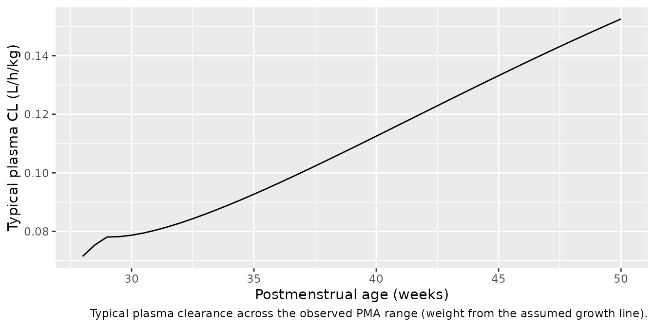

Assumptions and deviations

Maturation constants are not printed in the paper. The Methods state that all parameters were scaled a priori for size and age with a weight exponent of 0.632 and a maturation function on clearance, citing Germovsek et al. 2016 and 2017, but give no values. The maintainers used the pairing Germovsek et al. 2017 (Table 1, model 9b) gives for the fixed 0.632 exponent, PMA^3.33 / (55.4^3.33 + PMA^3.33) (the Rhodin 2009 glomerular-filtration fit with its estimated 0.632 exponent), which is also the pairing in the Germovsek 2016 gentamicin model the paper cites. The Rhodin constants paired with a 0.75 exponent (47.7 weeks, 3.4) would give a typical clearance about 45% higher at 34.4 weeks PMA, so this choice matters for plasma exposure.
No postnatal-age term. Germovsek 2016 also carried a gentamicin-specific postnatal-age factor with an estimated half-saturation. Table 3 lists no such estimate, so it is not included; at the cohort’s postnatal ages (3.9-23.1 weeks) that factor would be near 1 anyway.
Volume scales linearly with weight (exponent 1), inferred from Table 3 reporting V in L/70 kg.
CSF parameters are not weight- or age-scaled. Table 3 reports CLCSF in L/h and VCSF in L, without the per-70 kg normalisation used for the plasma parameters, and the Results describe no covariate on them.
IIV variances. The Table 3 footnote defines CV as 100 x omega, so each variance is (CV/100)^2. IIV on V was fixed to 0 and is omitted.
Current weight was not reported. Only birth weight is tabulated. The virtual cohort uses a linear growth assumption (1.6 kg at 34.4 weeks PMA, +0.18 kg per week, 12% scatter). This affects the plasma simulations only.
IV infusion duration was not reported. A 1-hour infusion is assumed. The paper gives intervals only up to 35 weeks PMA (every 12 h for 29-35 weeks); every virtual infant receives every-12-hour dosing.
CLCSF is printed to one significant figure (0.002 L/h; bootstrap median 0.002, 95% CI 0.002-0.003), so the CSF half-life of about 38 h carries that rounding.
Figure 3 (time to CSF sterilisation against CSF AUC0-24 and average concentration) is an exploratory scatter of observed outcomes with no fitted relationship, so it is not reproduced.
No erratum or correction notice was found for this article (checked 2026-09-27).