Rosuvastatin (Macpherson 2015)
Source:vignettes/articles/Macpherson_2015_rosuvastatin.Rmd
Macpherson_2015_rosuvastatin.RmdModel and source
- Citation: Macpherson M, Hamren B, Braamskamp MJAM, Kastelein JJP, Lundstrom T, Martin PD. Population pharmacokinetics of rosuvastatin in pediatric patients with heterozygous familial hypercholesterolemia. Eur J Clin Pharmacol. 2016;72(1):19-27. doi:10.1007/s00228-015-1946-4.
- Description: Two-compartment population PK model with first-order oral absorption for rosuvastatin in pediatric patients (aged 6 to <18 years) with heterozygous familial hypercholesterolemia (Macpherson 2015 Eur J Clin Pharmacol). Apparent clearance scales with body weight (estimated power exponent 0.352, reference 42 kg) and is 1.41-fold higher in males than females. Residual error is proportional and switches between intensive and sparse PK sampling phases.
- Article: Eur J Clin Pharmacol 2016;72(1):19-27. https://doi.org/10.1007/s00228-015-1946-4
Population
The model was developed in 214 pediatric patients with heterozygous familial hypercholesterolemia (HeFH), pooled from two AstraZeneca studies (Macpherson 2015 Table 1):
- CHARON (NCT01078675; n = 196): a phase 3 open-label multicenter 2-year safety / efficacy / PK study in patients aged 6 to <18 years. Initial dose was 5 mg once daily, titrated up to 20 mg (patients aged 10 to <18 years) or 10 mg (patients aged 6 to <10 years) if LDL-C target <110 mg/dL was not reached. Median (range) baseline weight 42.0 kg (20.0-111), age 11 years (6-17); 56% female; 90% Caucasian. 12 PK-pilot subjects (younger than Tanner stage II) received a single 10 mg dose with intensive 24-h sampling on Day 0; all 196 subjects then provided sparse pre-dose samples after the first month and every 3 months over 2 years (1,735 measurable concentrations total).
- Study 4522IL/0086 (n = 18): a single- and multiple-dose precursor study in children aged 10 to <18 years. Six subjects per dose group received a single oral dose of 10, 40, or 80 mg with intensive sampling at -0.5, 0.5, 1, 2, 3, 4, 5, 6, 9, 12, 18, 24, 48, 72, and 96 h post-dose. The 80 mg cohort additionally received 80 mg once daily for 7 days with intensive steady-state sampling at -0.5, 0.5, 1, 2, 3, 4, 5, 6, 9, 12, 18, and 24 h on Day 7. Median (range) baseline weight 63.2 kg (32-116), age 14 years (10-17); 50% female; 78% Caucasian.
The combined dataset yielded 2,029 measurable rosuvastatin
concentrations (CHARON LLOQ 0.02 ng/mL, range 0.02-20 ng/mL; 4522IL/0086
LLOQ 0.1 ng/mL, range 0.1-30 ng/mL). Race was not formally analyzed as a
covariate because 89% of patients were Caucasian and the frequency of
any other race was <7%. The same demographic information is available
programmatically via
readModelDb("Macpherson_2015_rosuvastatin")$population.
Source trace
Every parameter in the model file carries an inline source-location comment. The table below collects the entries in one place.
| Equation / parameter | Value | Source location |
|---|---|---|
lka (Ka absorption rate) |
0.183 1/h | Table 2, final-model column, Ka row (RSE 10.5%) |
lcl (CL/F at WT=42 kg, female) |
129 L/h | Table 2, final-model column, CL/F row (RSE 5.70%) |
lvc (Vc/F central volume) |
303 L | Table 2, final-model column, Vc/F row (RSE 28.0%) |
lq (Q/F intercompartmental clearance) |
89.9 L/h | Table 2, final-model column, Q/F row (RSE 15.6%) |
lvp (Vp/F peripheral volume) |
5,153 L | Table 2, final-model column, Vp/F row (RSE 23.9%) |
e_wt_cl (weight power exponent on CL/F) |
0.352 | Table 2, final-model column, Weight CL/F x (WT/42)^theta row (RSE 23.9%) |
e_sexf_cl (Male fold-effect on CL/F) |
1.41 | Table 2, final-model column, Male CL/F x theta row (RSE 6.33%) |
| IIV CL/F (omega^2 = log(1 + 0.40^2) = 0.14842) | 40.0% CV | Table 2, final-model column, IIV CL/F row (RSE 8.09%) |
| IIV Vc/F (omega^2 = log(1 + 1.05^2) = 0.74295) | 105% CV | Table 2, final-model column, IIV Vc/F row (RSE 15.5%) |
| IIV Q/F (omega^2 = log(1 + 0.648^2) = 0.35067) | 64.8% CV | Table 2, final-model column, IIV Q/F row (RSE 13.3%) |
propSdSparse (sparse residual error) |
59.5% CV | Table 2, final-model column, Residual error sparse sampling row (RSE 4.40%) |
propSdIntensive (intensive residual error) |
39.4% CV | Table 2, final-model column, Residual error intensive sampling row (RSE 7.89%) |
| Structural model: 2-cpt + first-order oral absorption + first-order elimination | – | Results, “Base model” / Figure (Supplemental Fig. 1) |
| Covariate equation: CL/F = 129 * (WT/42)^0.352 * 1.41^(1 - SEXF) | – | Final-model expression, p. 23 (Results, Final model paragraph) and Table 2 |
| Residual error split: proportional (additive on log scale), separated by intensive vs sparse sampling | – | Results, Base model paragraph 2 |
Virtual cohort
The published individual-subject data are not openly available. The virtual cohort below mirrors the intensive-sampling design of Study 4522IL/0086 (single 10, 40, or 80 mg oral dose, n = 6 per dose group per the source paper, scaled up to 200 subjects per dose for stable percentiles), with baseline demographics drawn from a uniform body weight distribution over the published range and a 50% sex split matching that study (Table 1).
set.seed(20150921)
n_per_dose <- 80L

make_cohort <- function(n, dose_mg, id_offset = 0L) {
  tibble(
    id   = id_offset + seq_len(n),
    WT   = runif(n, min = 32, max = 116),
    SEXF = sample(c(0L, 1L), size = n, replace = TRUE),
    dose_mg = dose_mg
  )
}

demo <- bind_rows(
  make_cohort(n_per_dose, dose_mg = 10L,  id_offset =          0L),
  make_cohort(n_per_dose, dose_mg = 40L,  id_offset =     n_per_dose),
  make_cohort(n_per_dose, dose_mg = 80L,  id_offset = 2L * n_per_dose)
) |>
  mutate(treatment = factor(paste0(dose_mg, " mg"),
                            levels = c("10 mg", "40 mg", "80 mg")))

stopifnot(!anyDuplicated(demo$id))
Simulation
Each subject receives a single oral dose at time 0 with the sampling
schedule used in Study 4522IL/0086 (Macpherson 2015 Methods, p. 21):
-0.5, 0.5, 1, 2, 3, 4, 5, 6, 9, 12, 18, 24, 48, 72, 96 h.
SAMPLE_INTENSIVE is set to 1 on every observation
(intensive sampling).
sample_times <- c(0, 0.5, 1, 2, 3, 4, 5, 6, 9, 12, 18, 24, 48, 72, 96)

build_events <- function(demo, obs_grid) {
  doses <- demo |>
    mutate(amt  = dose_mg,
           evid = 1L,
           cmt  = "depot",
           time = 0,
           SAMPLE_INTENSIVE = 1L) |>
    select(id, time, amt, evid, cmt, WT, SEXF, SAMPLE_INTENSIVE,
           treatment, dose_mg)
  obs <- demo |>
    select(id, WT, SEXF, treatment, dose_mg) |>
    tidyr::crossing(time = obs_grid) |>
    mutate(amt = NA_real_,
           evid = 0L,
           cmt  = NA_character_,
           SAMPLE_INTENSIVE = 1L)
  bind_rows(doses, obs) |>
    arrange(id, time, desc(evid))
}

events_paper <- build_events(demo, obs_grid = sample_times)
mod <- rxode2::rxode2(readModelDb("Macpherson_2015_rosuvastatin"))
#> ℹ parameter labels from comments will be replaced by 'label()'

sim_paper <- rxode2::rxSolve(mod, events = events_paper,
                             keep = c("treatment", "WT", "SEXF")) |>
  as.data.frame()
Replicate published figures
Figure 4b – single-dose intensive profiles, 4522IL/0086
Macpherson 2015 Figure 4b shows VPC envelopes for the three single-dose intensive cohorts (10, 40, 80 mg) from Study 4522IL/0086 over the 0-96 h window. The chunk below reproduces the 5th-50th-95th percentile envelope from the cohort-level simulation.
vpc_data <- sim_paper |>
  filter(time > 0) |>
  group_by(treatment, time) |>
  summarise(Q05 = quantile(Cc, 0.05, na.rm = TRUE),
            Q50 = quantile(Cc, 0.50, na.rm = TRUE),
            Q95 = quantile(Cc, 0.95, na.rm = TRUE),
            .groups = "drop")

ggplot(vpc_data, aes(time, Q50)) +
  geom_ribbon(aes(ymin = Q05, ymax = Q95), alpha = 0.3) +
  geom_line(linewidth = 0.7) +
  facet_wrap(~ treatment) +
  scale_x_continuous(breaks = seq(0, 96, by = 24)) +
  scale_y_log10() +
  labs(x = "Time post-dose (h)",
       y = "Rosuvastatin concentration (ng/mL, log scale)",
       title = "Stochastic VPC by single-dose cohort (Study 4522IL/0086)",
       caption = "Replicates Figure 4b of Macpherson 2015.")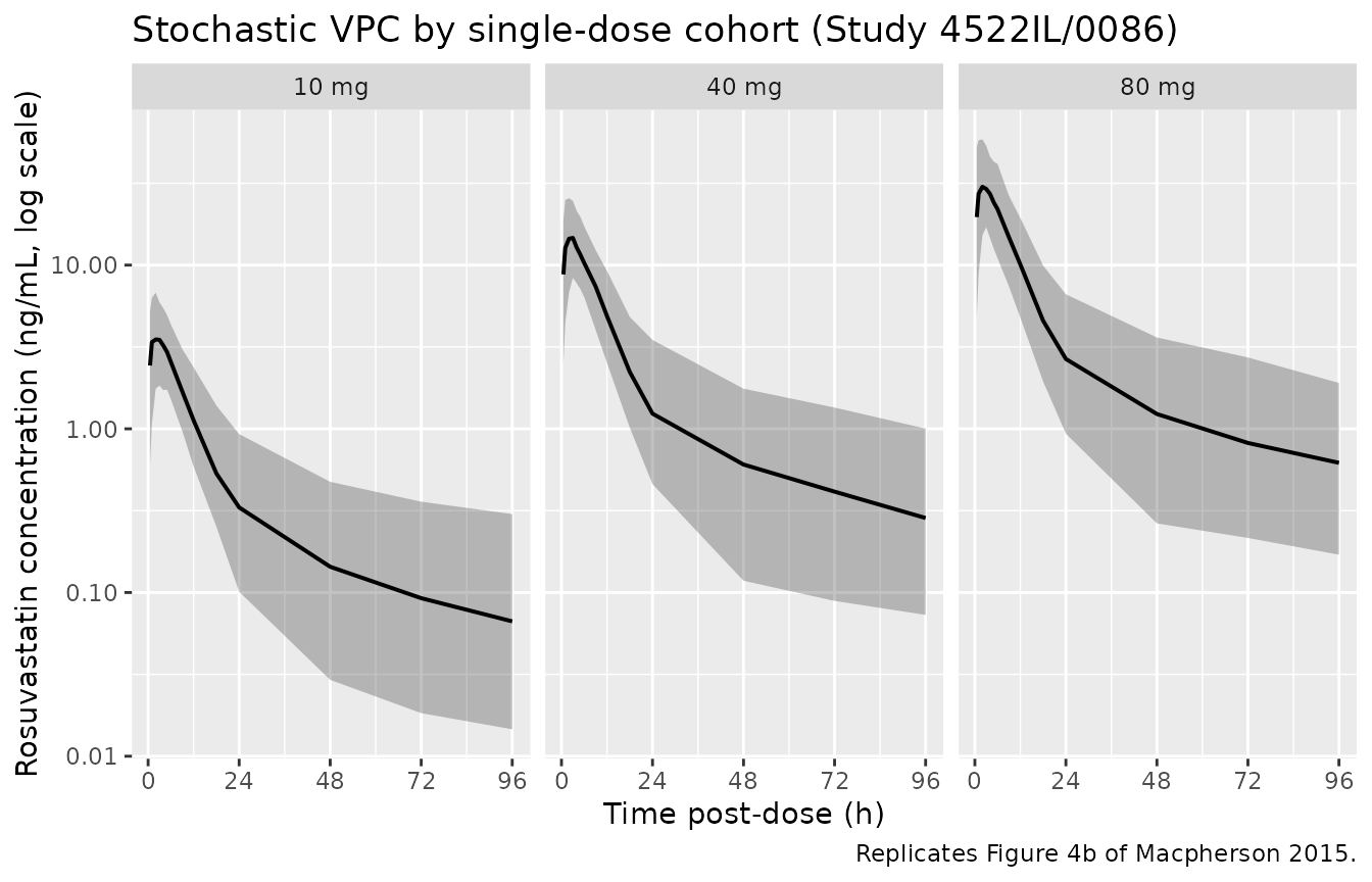
Replicates Figure 4b of Macpherson 2015: 5th-50th-95th percentile rosuvastatin concentration vs. time after a single oral dose, by dose group (200 subjects per dose group).
CL/F vs body weight and sex (Figure 2c, d)
Macpherson 2015 Figure 2c and 2d show individual CL/F estimates plotted against body weight and sex respectively. The figure below reproduces the typical-value covariate relationship from the packaged model: CL/F = 129 (WT/42)^0.352 1.41^(1 - SEXF), evaluated over the observed weight range.
cl_curve <- expand.grid(
  WT   = seq(20, 116, by = 1),
  SEXF = c(0L, 1L)
) |>
  mutate(
    sex_label = factor(ifelse(SEXF == 1L, "Female", "Male"),
                       levels = c("Female", "Male")),
    cl_f = 129 * (WT / 42)^0.352 * 1.41^(1 - SEXF)
  )

ggplot(cl_curve, aes(WT, cl_f, colour = sex_label)) +
  geom_line(linewidth = 0.7) +
  labs(x = "Body weight (kg)",
       y = "Typical CL/F (L/h)",
       colour = "Sex",
       title = "Typical CL/F vs body weight, stratified by sex",
       caption = "Replicates Figure 2c/d of Macpherson 2015 (typical-value covariate effect).")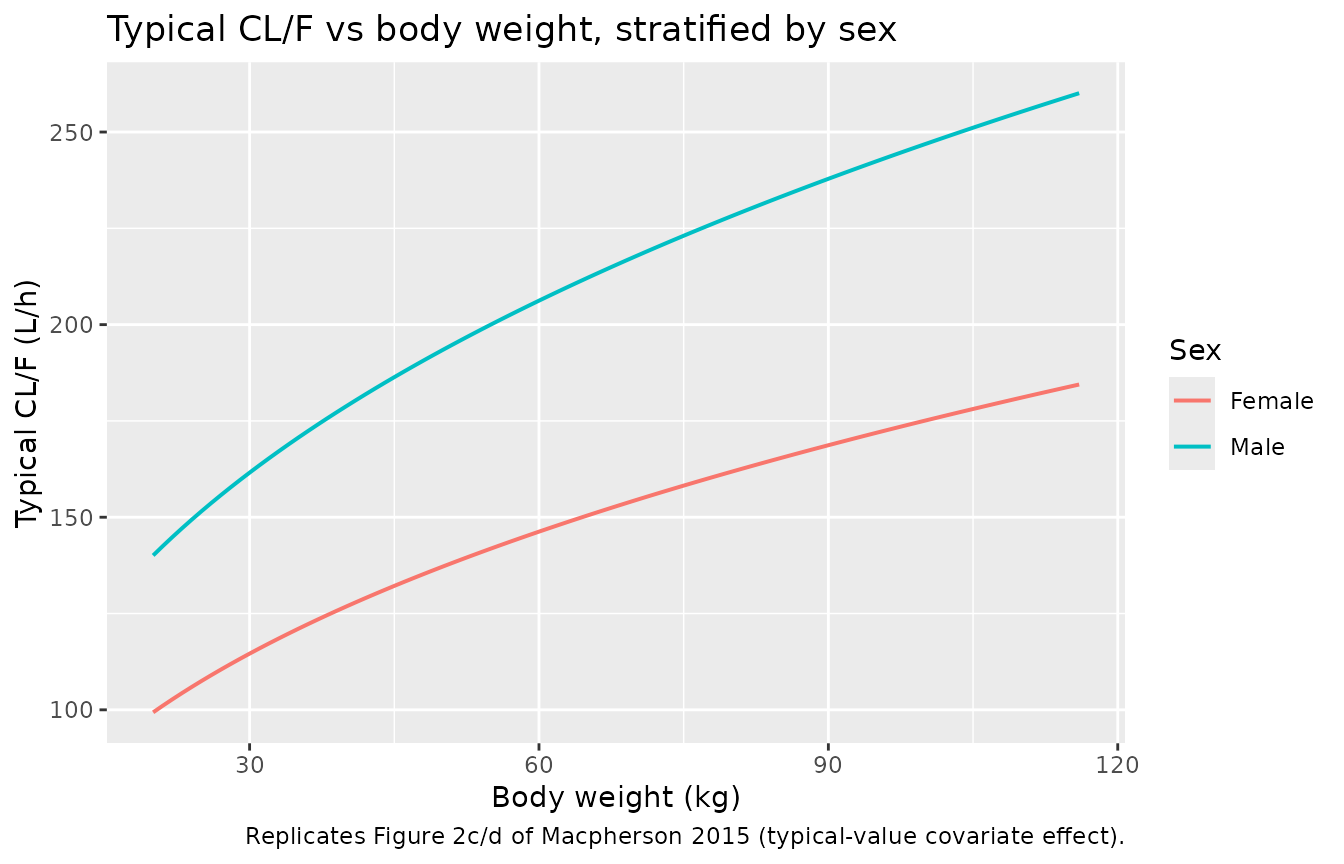
Replicates Figure 2c/d of Macpherson 2015: typical-value CL/F vs body weight, stratified by sex. Male children have CL/F ~1.41x higher than female children of the same weight.
PKNCA validation
PKNCA computes Cmax, Tmax, and AUClast / AUCinf for each subject across the three single-dose cohorts.
nca_input <- sim_paper |>
  select(id, time, Cc, treatment)

dose_df <- demo |>
  mutate(time = 0, amt = dose_mg) |>
  select(id, time, amt, treatment)

conc_obj <- PKNCA::PKNCAconc(nca_input, Cc ~ time | treatment + id,
                             concu = "ng/mL", timeu = "h")
dose_obj <- PKNCA::PKNCAdose(dose_df, amt ~ time | treatment + id,
                             doseu = "mg")
intervals <- data.frame(start      = 0,
                        end        = 96,
                        cmax       = TRUE,
                        tmax       = TRUE,
                        auclast    = TRUE,
                        aucinf.obs = TRUE,
                        half.life  = TRUE)
nca_data <- PKNCA::PKNCAdata(conc_obj, dose_obj, intervals = intervals)
nca_res  <- suppressMessages(suppressWarnings(PKNCA::pk.nca(nca_data)))
nca_summary <- summary(nca_res)
knitr::kable(nca_summary,
caption = "Simulated NCA parameters by single-dose cohort (200 subjects per dose, Study 4522IL/0086 sampling schedule).")| Interval Start | Interval End | treatment | N | AUClast (h*ng/mL) | Cmax (ng/mL) | Tmax (h) | Half-life (h) | AUCinf,obs (h*ng/mL) |
|---|---|---|---|---|---|---|---|---|
| 0 | 96 | 10 mg | 80 | 46.0 [37.3] | 3.87 [37.1] | 2.00 [1.00, 9.00] | 63.5 [21.6] | 51.8 [43.3] |
| 0 | 96 | 40 mg | 80 | 192 [42.8] | 16.1 [34.7] | 2.00 [0.500, 9.00] | 62.0 [21.8] | 218 [50.0] |
| 0 | 96 | 80 mg | 80 | 400 [40.5] | 34.6 [34.6] | 2.00 [0.500, 9.00] | 62.3 [22.0] | 458 [48.2] |
Dose proportionality check
Rosuvastatin PK was reported as linear in dose (Results, Base model paragraph 4: “CL/F was independent of dose”). The chunk below verifies that the median simulated AUCinf scales linearly with dose across the 10 / 40 / 80 mg cohorts.
auc_long <- as.data.frame(nca_res$result) |>
  filter(PPTESTCD == "aucinf.obs")

auc_by_dose <- auc_long |>
  inner_join(demo |> select(id, dose_mg), by = "id") |>
  group_by(treatment, dose_mg) |>
  summarise(median_auc = median(PPORRES, na.rm = TRUE),
            q05        = quantile(PPORRES, 0.05, na.rm = TRUE),
            q95        = quantile(PPORRES, 0.95, na.rm = TRUE),
            .groups    = "drop") |>
  mutate(auc_per_mg = median_auc / dose_mg)

knitr::kable(auc_by_dose,
caption = "Median simulated AUCinf by dose, with the dose-normalised AUCinf/mg column verifying dose linearity.")| treatment | dose_mg | median_auc | q05 | q95 | auc_per_mg |
|---|---|---|---|---|---|
| 10 mg | 10 | 50.70489 | 25.98403 | 103.0506 | 5.070489 |
| 40 mg | 40 | 220.17752 | 105.22929 | 390.3965 | 5.504438 |
| 80 mg | 80 | 444.81679 | 219.63401 | 926.3404 | 5.560210 |
The dose-normalised AUCinf/mg column should be approximately constant across cohorts; large departures indicate a structural mismatch and would warrant investigation rather than parameter tuning.
Assumptions and deviations
- Race not modelled. The paper did not formally analyse race as a covariate because 89% of patients were Caucasian and any other race category was <7% (Results, Covariate analysis paragraph 3). The packaged model therefore carries no race covariate; downstream users simulating non-Caucasian-dominated cohorts should treat the predictions accordingly.
-
Age not modelled. Age was tested as a linear
function of CL/F and dropped from the final model: the gradient was
poorly estimated (0.043, RSE 108%) and weight + sex explained the
apparent age effect (Results, Covariate analysis paragraph 5). Age also
did not enter as a maturation function in the published model. The paper
noted a small ~16% increase in CL/F over the 2-year CHARON treatment
period, which was tracked through time-varying body weight rather than
an explicit time-on-treatment effect; the packaged model captures this
via the time-varying
WTcovariate. -
No IIV on Ka or Vp/F. The published final model
estimated IIV on CL/F, Vc/F, and Q/F only (Table 2). The packaged
ini()mirrors that choice; downstream users wishing to perturb absorption or peripheral volume must add IIV terms manually. - Covariate sign convention for sex. The paper reports Male CL/F x 1.41 with female children as the implicit reference, so the model encodes the factor as 1.41^(1 - SEXF) to keep the published structural CL/F = 129 L/h interpretable as the female-at-42-kg typical value. Table 2’s worked numerical examples (140 L/h for a 20 kg male, 99 L/h for a 20 kg female, 246 L/h for a 99 kg male, 182 L/h for a 111 kg female) reproduce exactly under this encoding.
-
SAMPLE_INTENSIVEindicator added to the canonical covariate register. Macpherson 2015 estimated two residual-error magnitudes separated by sampling intensity (39.4% CV intensive vs 59.5% CV sparse; Table 2). The packaged model carries both and switches them via the per-observationSAMPLE_INTENSIVEindicator, following the established pattern of per-record residual-error switches in nlmixr2lib (STUDY1/STUDY5inCirincione_2017_exenatide.R,ELISAinValenzuela_2025_nipocalimab.R,STUDY_NIPOCALIMAB_PHASE1in the same). The new entry is documented ininst/references/covariate-columns.mdwith general scope. -
Vignette focuses on intensive single-dose sampling.
The intensive 4522IL/0086 single-dose cohorts give the cleanest VPC
comparison against Macpherson 2015 Figure 4b. CHARON sparse pre-dose
troughs (the bulk of the published dataset) are not separately
reproduced here because they occur at irregular randomised times that
the source paper does not publish at the per-subject level. Users
wishing to reproduce the CHARON sparse VPC (Figure 4a) should set
SAMPLE_INTENSIVE = 0and simulate pre-dose troughs at their own visit schedule. - Vignette uses 80 subjects per dose group. The source paper had 6 subjects per dose group in Study 4522IL/0086 (Methods); we scale up to 80 for stable VPC percentiles while keeping the vignette inside the 5-minute pkgdown render budget.
-
Year 2015 in the filename / function name.
Published online 21 September 2015 (DOI 10.1007/s00228-015-1946-4);
print issue is Eur J Clin Pharmacol 72(1):19-27 (January 2016). The
filename and
Macpherson_2015_rosuvastatinfunction name use the online-first year; thereferencestring and the source-trace table cite the print-issue year for clarity.