Hydroxychloroquine in COVID-19 (Themans 2020)
Source:vignettes/articles/Themans_2020_hydroxychloroquine.Rmd
Themans_2020_hydroxychloroquine.RmdModel and source
- Citation: Themans P, Belkhir L, Dauby N, Yombi JC, De Greef J, Delongie KA, Vandeputte M, Nasreddine R, Wittebole X, Wuillaume F, Lescrainier C, Verlinden V, Kiridis S, Dogne JM, Hamdani J, Wallemacq P, Musuamba FT. Population Pharmacokinetics of Hydroxychloroquine in COVID-19 Patients: Implications for Dose Optimization. Eur J Drug Metab Pharmacokinet. 2020;45:703-713. doi:10.1007/s13318-020-00648-y. PMCID PMC7511144.
- Description: One-compartment first-order-absorption population PK model for oral hydroxychloroquine (HCQ) whole-blood concentrations in 48 hospitalised adult COVID-19 patients from two Belgian tertiary hospitals, with bioavailability fixed at 0.746 from Carmichael 2003 and a power (allometric-type) body-weight effect on clearance (Themans 2020).
- Article: https://doi.org/10.1007/s13318-020-00648-y
Population
Themans 2020 modelled 84 whole-blood hydroxychloroquine (HCQ) concentrations from hospitalised adults with COVID-19 at two tertiary hospitals in Brussels, Belgium (Section 2.1 and Table 1). The model-building dataset had 48 patients: 33 from an open-label single-arm study (Eudract 2020-001434-35) and 15 treated as standard of care. Eight more standard-of-care patients were held out for external validation. The model-building cohort was 26 male and 22 female, with median age 58.5 years (range 21-93) and median weight 80 kg (range 50-122; two missing values were imputed to the median). Patients received the Belgian national protocol: 400 mg HCQ sulfate twice daily on day 1, then 200 mg twice daily for a 5-day course. Plaquenil 200 mg sulfate tablets contain 155 mg HCQ base. Sampling was sparse: one opportunistic sample within 4 h of a dose, and one at the end of treatment.
Source trace
| Element | Value | Source |
|---|---|---|
| Structure | 1-compartment, first-order absorption and elimination, no lag | Results paragraph 1 |
lka |
log(9.3) 1/h | Table 2 |
lcl |
log(15.7) L/h at 80 kg | Table 2 |
lvc |
log(860.8) L | Table 2 |
lfdepot |
fixed(log(0.746)) | Table 2 (fixed, from Carmichael 2003) |
e_wt_cl |
1.38 | Table 2 ‘WT effect on CL’ |
| WT form | CL * (WT/COV_POP)^theta2 * exp(eta) |
Eq. 1 |
| COV_POP | 80 kg (not printed) | Table 1 median; checked against Table S1 below |
etalcl |
0.15 | Table 2 omega^2 |
etalvc |
0.27 | Table 2 omega^2 |
propSd |
sqrt(0.029) = 0.1703 | Table 2 sigma^2 |
| Dose unit | mg HCQ base | Section 2.1; checked against Table S1 below |
| Observation | whole blood, ng/mL | Section 2.2 |
mod <- readModelDb("Themans_2020_hydroxychloroquine")
mod_typ <- rxode2::zeroRe(mod)
#> ℹ parameter labels from comments will be replaced by 'label()'
Dosing regimens
The regimens in Figure 5 and Supplementary Table S1 are written as mg HCQ sulfate. They are converted to mg base (x 155/200) for the model.
salt_to_base <- 155 / 200

# Day-1 loading doses (times in h, amounts in mg sulfate), then maintenance
# from 24 h at `md` mg every `tau` h until the end of treatment.
regimen_table <- tibble::tribble(
  ~regimen, ~ld_times, ~ld_amts, ~md, ~tau,
  "Blue: 400 mg BID D1, 200 mg BID", c(0, 12), c(400, 400), 200, 12,
  "Orange: 800/800/400 mg D1, 400 mg BID", c(0, 6, 12), c(800, 800, 400), 400, 12,
  "Yellow: 600 mg BID D1, 200 mg BID", c(0, 12), c(600, 600), 200, 12,
  "Purple: 200 mg TID D1, 200 mg BID", c(0, 8, 16), c(200, 200, 200), 200, 12,
  "Green: 200 mg BID", c(0, 12), c(200, 200), 200, 12,
  "Black-red: 400 mg BID D1, 400 mg QD", c(0, 12), c(400, 400), 400, 24
)

dose_schedule <- function(i, days) {
  r <- regimen_table[i, ]
  mt <- seq(24, 24 * days - 1, by = r$tau)
  data.frame(
    time = c(r$ld_times[[1]], mt),
    amt = salt_to_base * c(r$ld_amts[[1]], rep(r$md, length(mt)))
  )
}
Typical-value profiles (Figure 5)
obs_times <- seq(0, 240, by = 1)
fig5 <- list()
for (i in seq_len(nrow(regimen_table))) {
  for (days in c(5, 10)) {
    for (wt in c(50, 150)) {
      d <- dose_schedule(i, days)
      ev <- dplyr::bind_rows(
        data.frame(id = 1L, time = d$time, amt = d$amt, evid = 1L, cmt = "depot"),
        data.frame(id = 1L, time = obs_times, amt = 0, evid = 0L, cmt = "central")
      ) |>
        dplyr::arrange(time, dplyr::desc(evid)) |>
        dplyr::mutate(WT = wt)
      s <- as.data.frame(rxode2::rxSolve(mod_typ, ev, returnType = "data.frame"))
      fig5[[length(fig5) + 1]] <- data.frame(
        time = s$time, Cc = s$Cc, WT = paste(wt, "kg"),
        regimen = regimen_table$regimen[i], duration = paste(days, "days")
      )
    }
  }
}
#> ℹ omega/sigma items treated as zero: 'etalcl', 'etalvc'
#> ℹ omega/sigma items treated as zero: 'etalcl', 'etalvc'
#> ℹ omega/sigma items treated as zero: 'etalcl', 'etalvc'
#> ℹ omega/sigma items treated as zero: 'etalcl', 'etalvc'
#> ℹ omega/sigma items treated as zero: 'etalcl', 'etalvc'
#> ℹ omega/sigma items treated as zero: 'etalcl', 'etalvc'
#> ℹ omega/sigma items treated as zero: 'etalcl', 'etalvc'
#> ℹ omega/sigma items treated as zero: 'etalcl', 'etalvc'
#> ℹ omega/sigma items treated as zero: 'etalcl', 'etalvc'
#> ℹ omega/sigma items treated as zero: 'etalcl', 'etalvc'
#> ℹ omega/sigma items treated as zero: 'etalcl', 'etalvc'
#> ℹ omega/sigma items treated as zero: 'etalcl', 'etalvc'
#> ℹ omega/sigma items treated as zero: 'etalcl', 'etalvc'
#> ℹ omega/sigma items treated as zero: 'etalcl', 'etalvc'
#> ℹ omega/sigma items treated as zero: 'etalcl', 'etalvc'
#> ℹ omega/sigma items treated as zero: 'etalcl', 'etalvc'
#> ℹ omega/sigma items treated as zero: 'etalcl', 'etalvc'
#> ℹ omega/sigma items treated as zero: 'etalcl', 'etalvc'
#> ℹ omega/sigma items treated as zero: 'etalcl', 'etalvc'
#> ℹ omega/sigma items treated as zero: 'etalcl', 'etalvc'
#> ℹ omega/sigma items treated as zero: 'etalcl', 'etalvc'
#> ℹ omega/sigma items treated as zero: 'etalcl', 'etalvc'
#> ℹ omega/sigma items treated as zero: 'etalcl', 'etalvc'
#> ℹ omega/sigma items treated as zero: 'etalcl', 'etalvc'
fig5 <- dplyr::bind_rows(fig5)

ggplot(fig5, aes(time / 24, Cc, colour = regimen, linetype = duration)) +
  geom_line() +
  geom_hline(yintercept = 0.72 / 0.5 / 0.53 * 335.87, colour = "grey40") +
  facet_wrap(~WT) +
  labs(x = "Time (days)", y = "HCQ whole-blood concentration (ng/mL)", colour = NULL, linetype = NULL) +
  theme_bw() +
  theme(legend.position = "bottom", legend.direction = "vertical")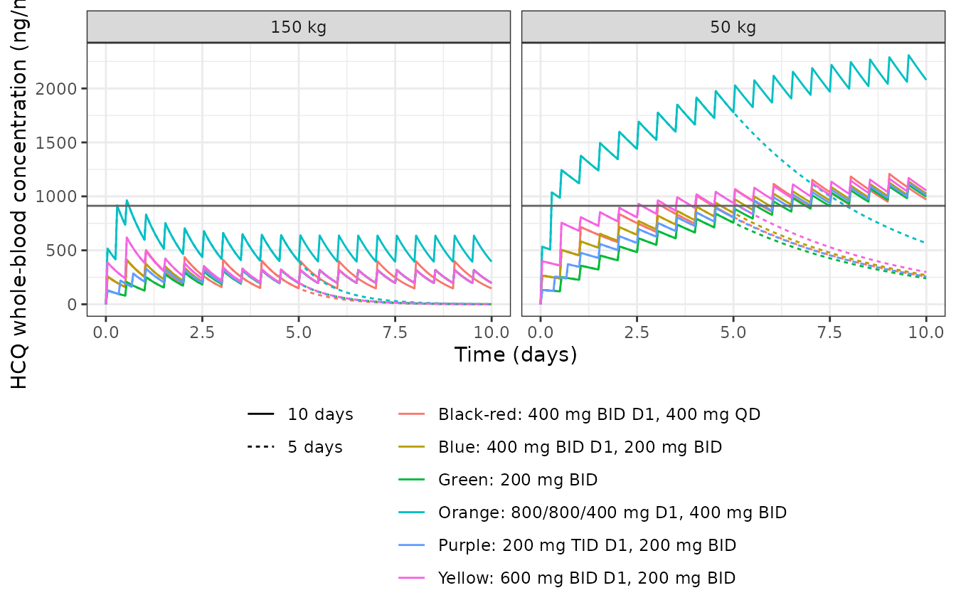
Replicates the median curves of Figure 5 of Themans 2020 (typical values; the grey line is the whole-blood target from the Yao EC50, derived below).
Clearance versus weight (Figure 4)
wt_grid <- seq(50, 150, by = 1)
ggplot(data.frame(WT = wt_grid, CL = 15.7 * (wt_grid / 80)^1.38), aes(WT, CL)) +
  geom_line() +
  labs(x = "Body weight (kg)", y = "Typical CL (L/h)") +
  theme_bw()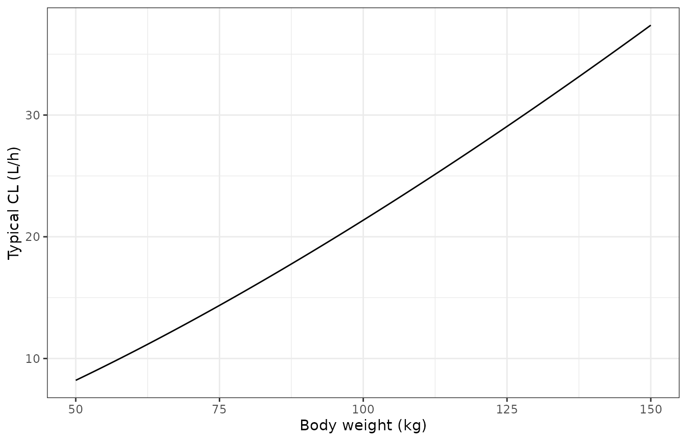
Typical-value counterpart of the post hoc clearances in Figure 4.
Reproducing Supplementary Table S1
Table S1 reports the percentage of simulated 50 kg and 150 kg patients whose whole-blood concentration at the end of treatment exceeds a target. For the Yao EC50 (0.72 uM), the paper scales the free plasma EC50 to total whole blood with 50% protein binding and a serum/whole-blood ratio of 0.53 (Discussion). With the HCQ base molar mass of 335.87 g/mol this gives 0.72 / 0.5 / 0.53 x 335.87 = 913 ng/mL. The Liu EC50 (4.51 uM) gives about 5700 ng/mL, and every cell for it is 0% in the paper.
The paper used 1000 Monte Carlo subjects per scenario. Here the
probability is computed deterministically instead: a quantile grid over
etalcl and etalvc, closed-form one-compartment
superposition, and the proportional residual error integrated
analytically. First, the closed form is checked against
rxSolve().
conc_closed <- function(t, dosing, cl, v, ka = 9.3, f = 0.746) {
  k <- cl / v
  out <- 0
  for (j in seq_len(nrow(dosing))) {
    dt <- t - dosing$time[j]
    if (dt > 0) {
      out <- out + 1000 * f * dosing$amt[j] * ka / (v * (ka - k)) * (exp(-k * dt) - exp(-ka * dt))
    }
  }
  out
}

chk <- fig5 |>
  dplyr::filter(WT == "50 kg", duration == "5 days", time %in% c(6, 50, 120, 200)) |>
  dplyr::mutate(
    i = match(regimen, regimen_table$regimen),
    closed = mapply(function(tt, ii) conc_closed(tt, dose_schedule(ii, 5), 15.7 * (50 / 80)^1.38, 860.8), time, i)
  )
stopifnot(all(abs(chk$Cc / chk$closed - 1) < 1e-4))
target_yao <- 0.72 / 0.5 / 0.53 * 335.87
k_grid <- 150
z <- stats::qnorm((seq_len(k_grid) - 0.5) / k_grid)
grid <- expand.grid(zcl = z, zv = z)

pta <- function(i, days, wt, wt_ref = 80, dose_factor = 1) {
  d <- dose_schedule(i, days)
  d$amt <- d$amt * dose_factor
  cl <- 15.7 * (wt / wt_ref)^1.38 * exp(sqrt(0.15) * grid$zcl)
  v <- 860.8 * exp(sqrt(0.27) * grid$zv)
  cc <- conc_closed(24 * days, d, cl, v)
  # P(cc * (1 + eps) > target), eps ~ N(0, 0.029)
  100 * mean(1 - stats::pnorm((target_yao / cc - 1) / sqrt(0.029)))
}

published <- tibble::tribble(
  ~i, ~days, ~pub50, ~pub150,
  1, 5, 34.4, 0, 1, 10, 55.8, 0.1,
  2, 5, 93.3, 2.7, 2, 10, 96.1, 3.4,
  3, 5, 43.3, 0, 3, 10, 57.9, 0.1,
  4, 5, 29.2, 0, 4, 10, 54.3, 0.1,
  5, 5, 21.7, 0, 5, 10, 50.1, 0,
  6, 5, 28.7, 0, 6, 10, 48.9, 0.1
)

s1 <- published |>
  dplyr::rowwise() |>
  dplyr::mutate(
    sim50 = pta(i, days, 50),
    sim150 = pta(i, days, 150),
    sim50_ref70 = pta(i, days, 50, wt_ref = 70),
    sim50_salt = pta(i, days, 50, dose_factor = 1 / salt_to_base)
  ) |>
  dplyr::ungroup() |>
  dplyr::mutate(regimen = regimen_table$regimen[i])

s1 |>
  dplyr::select(regimen, days, pub50, sim50, pub150, sim150, sim50_ref70, sim50_salt) |>
  dplyr::rename(
    "Regimen" = regimen, "Days" = days,
    "50 kg, paper (%)" = pub50, "50 kg, model (%)" = sim50,
    "150 kg, paper (%)" = pub150, "150 kg, model (%)" = sim150,
    "50 kg, WT/70 (%)" = sim50_ref70, "50 kg, salt dose (%)" = sim50_salt
  ) |>
knitr::kable(digits = 1)| Regimen | Days | 50 kg, paper (%) | 50 kg, model (%) | 150 kg, paper (%) | 150 kg, model (%) | 50 kg, WT/70 (%) | 50 kg, salt dose (%) |
|---|---|---|---|---|---|---|---|
| Blue: 400 mg BID D1, 200 mg BID | 5 | 34.4 | 32.0 | 0.0 | 0.0 | 21.4 | 58.5 |
| Blue: 400 mg BID D1, 200 mg BID | 10 | 55.8 | 52.9 | 0.1 | 0.0 | 37.4 | 76.4 |
| Orange: 800/800/400 mg D1, 400 mg BID | 5 | 93.3 | 92.7 | 2.7 | 3.4 | 87.1 | 98.1 |
| Orange: 800/800/400 mg D1, 400 mg BID | 10 | 96.1 | 96.2 | 3.4 | 3.9 | 91.4 | 99.0 |
| Yellow: 600 mg BID D1, 200 mg BID | 5 | 43.3 | 41.8 | 0.0 | 0.0 | 29.3 | 68.0 |
| Yellow: 600 mg BID D1, 200 mg BID | 10 | 57.9 | 55.9 | 0.1 | 0.0 | 40.1 | 78.3 |
| Purple: 200 mg TID D1, 200 mg BID | 5 | 29.2 | 27.4 | 0.0 | 0.0 | 18.0 | 53.4 |
| Purple: 200 mg TID D1, 200 mg BID | 10 | 54.3 | 51.4 | 0.1 | 0.0 | 36.2 | 75.4 |
| Green: 200 mg BID | 5 | 21.7 | 22.5 | 0.0 | 0.0 | 14.4 | 47.3 |
| Green: 200 mg BID | 10 | 50.1 | 49.7 | 0.0 | 0.0 | 34.8 | 74.2 |
| Black-red: 400 mg BID D1, 400 mg QD | 5 | 28.7 | 26.7 | 0.0 | 0.0 | 16.8 | 52.4 |
| Black-red: 400 mg BID D1, 400 mg QD | 10 | 48.9 | 46.5 | 0.1 | 0.0 | 31.2 | 70.4 |
stopifnot(
  # Monte Carlo noise on the paper's 1000-subject estimates is about 1.5
  # percentage points; the deterministic model values sit within 3.
  max(abs(s1$sim50 - s1$pub50)) < 4,
  max(abs(s1$sim150 - s1$pub150)) < 4,
  # The two alternatives are rejected: centring on 70 kg or dosing in mg
  # sulfate both miss the 5-day blue cell by more than 10 points.
  abs(s1$sim50_ref70[1] - s1$pub50[1]) > 10,
  abs(s1$sim50_salt[1] - s1$pub50[1]) > 10
)
The model reproduces all 24 Table S1 cells for the Yao target within 3 percentage points. The last two columns show why the reference weight is 80 kg and why the dose is in mg HCQ base. Centring on 70 kg lowers the 50 kg probabilities by 5 to 18 points. Dosing the sulfate amount raises them by 20 to 26 points, except for the orange regimen, which is already close to 100%. Centring on 81.5 kg (the median of all 56 patients) cannot be told apart from 80 kg at this precision. 80 kg is used because it is the model-building median and the weight split in Figures 2, 6 and S1.
Stochastic cohort under the Belgian protocol
rxode2::rxSetSeed(20200923)
n_sub <- 200
wt <- numeric(0)
while (length(wt) < n_sub) {
  draw <- stats::rlnorm(n_sub, log(80), 0.22)
  wt <- c(wt, draw[draw >= 50 & draw <= 122])
}
wt <- wt[seq_len(n_sub)]

d <- dose_schedule(1, 5)
ev_vpc <- dplyr::bind_rows(lapply(seq_len(n_sub), function(id) {
  dplyr::bind_rows(
    data.frame(id = id, time = d$time, amt = d$amt, evid = 1L, cmt = "depot"),
    data.frame(id = id, time = seq(0, 168, by = 2), amt = 0, evid = 0L, cmt = "central")
  ) |>
    dplyr::mutate(WT = wt[id])
})) |>
  dplyr::arrange(id, time, dplyr::desc(evid))

sim_vpc <- as.data.frame(rxode2::rxSolve(mod, ev_vpc, returnType = "data.frame"))
#> ℹ parameter labels from comments will be replaced by 'label()'

sim_vpc |>
  dplyr::group_by(time) |>
  dplyr::summarise(
    p05 = stats::quantile(sim, 0.05), p50 = stats::median(sim), p95 = stats::quantile(sim, 0.95)
  ) |>
  ggplot(aes(time / 24)) +
  geom_ribbon(aes(ymin = p05, ymax = p95), alpha = 0.3) +
  geom_line(aes(y = p50)) +
  labs(x = "Time (days)", y = "HCQ whole-blood concentration (ng/mL)") +
  theme_bw()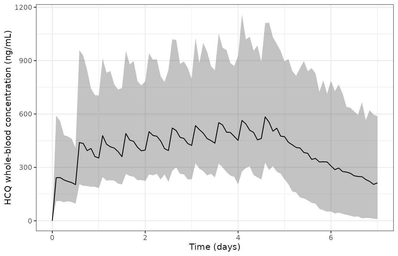
Median and 90% prediction interval for 200 virtual patients (weight 50-122 kg, centred at 80 kg) on the Belgian protocol. It is the model-side counterpart of Figure 3 and Figure S1.
PKNCA validation
A single 200 mg sulfate (155 mg base) dose is simulated for typical patients of 50, 80 and 150 kg. For a one-compartment model, AUC0-inf must equal F x Dose / CL and the half-life must equal ln(2) x V / CL.
wts <- c(50, 80, 150)
# Sample each weight out to 10 typical half-lives; beyond that the
# concentrations are solver noise and spoil the lambda-z fit.
t_end <- 10 * log(2) * 860.8 / (15.7 * (wts / 80)^1.38)
ev_nca <- dplyr::bind_rows(lapply(seq_along(wts), function(id) {
  t_nca <- c(0, 0.1, 0.25, 0.5, 1, 2, 4, 8, 12, seq(24, t_end[id], length.out = 40))
  dplyr::bind_rows(
    data.frame(id = id, time = 0, amt = 155, evid = 1L, cmt = "depot"),
    data.frame(id = id, time = t_nca, amt = 0, evid = 0L, cmt = "central")
  ) |>
    dplyr::mutate(WT = wts[id])
}))
sim_nca <- as.data.frame(rxode2::rxSolve(mod_typ, ev_nca, returnType = "data.frame", keep = "WT")) |>
  dplyr::mutate(treatment = paste(WT, "kg"))
#> ℹ omega/sigma items treated as zero: 'etalcl', 'etalvc'
#> Warning: multi-subject simulation without without 'omega'

conc_obj <- PKNCA::PKNCAconc(dplyr::filter(sim_nca, !is.na(Cc)), Cc ~ time | treatment + id)
dose_obj <- PKNCA::PKNCAdose(
  dplyr::distinct(sim_nca, id, treatment) |> dplyr::mutate(time = 0, amt = 155),
  amt ~ time | treatment + id
)
intervals <- data.frame(start = 0, end = Inf, cmax = TRUE, tmax = TRUE, aucinf.obs = TRUE, half.life = TRUE)
nca <- PKNCA::pk.nca(PKNCA::PKNCAdata(conc_obj, dose_obj, intervals = intervals))

nca_wide <- as.data.frame(nca$result) |>
  dplyr::filter(PPTESTCD %in% c("cmax", "tmax", "aucinf.obs", "half.life")) |>
  dplyr::select(treatment, PPTESTCD, PPORRES) |>
  tidyr::pivot_wider(names_from = PPTESTCD, values_from = PPORRES) |>
  dplyr::mutate(
    WT = as.numeric(sub(" kg", "", treatment)),
    cl = 15.7 * (WT / 80)^1.38,
    auc_theory = 1000 * 0.746 * 155 / cl,
    thalf_theory = log(2) * 860.8 / cl
  )

nca_wide |>
  dplyr::select(treatment, cmax, tmax, aucinf.obs, auc_theory, half.life, thalf_theory) |>
  dplyr::rename(
    "Weight" = treatment, "Cmax (ng/mL)" = cmax, "Tmax (h)" = tmax,
    "AUC0-inf (ng*h/mL)" = aucinf.obs, "F*Dose/CL" = auc_theory,
    "t1/2 (h)" = half.life, "ln2*V/CL" = thalf_theory
  ) |>
knitr::kable(digits = 1)| Weight | Cmax (ng/mL) | Tmax (h) | AUC0-inf (ng*h/mL) | F*Dose/CL | t1/2 (h) | ln2*V/CL |
|---|---|---|---|---|---|---|
| 150 kg | 130.8 | 0.5 | 3091.3 | 3093.4 | 16.0 | 16.0 |
| 50 kg | 133.2 | 1.0 | 14086.2 | 14088.2 | 72.7 | 72.7 |
| 80 kg | 132.1 | 1.0 | 7362.9 | 7365.0 | 38.0 | 38.0 |
stopifnot(
  all(abs(nca_wide$aucinf.obs / nca_wide$auc_theory - 1) < 0.02),
  all(abs(nca_wide$half.life / nca_wide$thalf_theory - 1) < 0.02)
)
The paper reports no NCA values, so the check is against the model’s own closed-form identities.
Assumptions and deviations
- Reference weight. Eq. 1 centres weight on a “population typical value” that is not printed. 80 kg is used: the model-building median (Table 1) and the weight split in the paper’s figures. Supplementary Table S1 is reproduced with 80 kg and rejects 70 kg (see above). The paper’s code was deposited in the DDMoRe Model Repository (DDMODEL00000322), which was unavailable when checked on 2026-09-27.
- Dose units. Doses enter the model as mg HCQ base (200 mg sulfate = 155 mg base), which reproduces Table S1. Dosing the sulfate amount does not.
- Bioavailability. Table 2 gives F = 0.746 (fixed); the abstract rounds it to 0.74. 0.746 is used, the Carmichael 2003 value it was taken from.
- Yellow regimen. Table S1 labels the day-1 dose as 600 mg TID, while the Figure 5 caption says 600 mg BID. The BID reading reproduces Table S1 (model 41.8% and 55.9% against the paper’s 43.3% and 57.9% for 50 kg); TID gives 56% for 5 days.
- Target concentration. The Table S1 target was re-derived from the Discussion’s scaling (50% protein binding, serum/whole-blood ratio 0.53) and the HCQ base molar mass; the paper does not print the resulting value.
- Time of the target check. “At the end of the treatment” is read as 24 x (number of days) hours after the first dose.
- Covariates not retained. Sex (correlated with weight) and age were tested on clearance but are not in the final model.