Amoxicillin + monophosphoryl lipid A in murine pneumococcal pneumonia (Franck 2021) • nlmixr2lib

Model and source

Franck et al. (2021) analysed pooled mouse studies of oral amoxicillin (AMX), the toll-like receptor 4 agonist monophosphoryl lipid A (MPLA), and their combination against Streptococcus pneumoniae serotype 1 pneumonia. The analysis was sequential, and the library reproduces it as two model files:

Franck_2021_amoxicillin_mouse – the stand-alone PK submodel (Supplementary Table S1): two compartments, first-order absorption after a lag time, interindividual variability on CL and Q, and an MPLA x dose interaction on clearance.
Franck_2021_amoxicillin_mpla_mouse – the pharmacometric PK/PD model of Table 1 with the PK fixed at those typical values, plus the survival (time-to-event) model of Table 2 linked through the model-predicted time of serum AMX above the MIC.

pk_ui <- rxode2::rxode(readModelDb("Franck_2021_amoxicillin_mouse"))
#> ℹ parameter labels from comments will be replaced by 'label()'
pd_ui <- rxode2::rxode(readModelDb("Franck_2021_amoxicillin_mpla_mouse"))

Citation: Franck S, Michelet R, Casilag F, Sirard JC, Wicha SG, Kloft C. A Model-Based Pharmacokinetic/Pharmacodynamic Analysis of the Combination of Amoxicillin and Monophosphoryl Lipid A Against S. pneumoniae in Mice. Pharmaceutics. 2021;13(4):469. doi:10.3390/pharmaceutics13040469. PK/PD parameters from Table 1, survival parameters from Table 2, equations from Supplementary Section S2 (Eqs. 1-7) and Figure 1.
PK submodel: Preclinical (mouse). Two-compartment population PK submodel for oral amoxicillin in mice infected intranasally with Streptococcus pneumoniae serotype 1 (Franck 2021), with first-order absorption after a lag time, first-order elimination, and a pharmacokinetic interaction in which intraperitoneal monophosphoryl lipid A (MPLA, 2 mg/kg) coadministration lowers amoxicillin clearance linearly with the amoxicillin dose (CL = 124 - 0.145 * dose in ug; -40.9% at 14 mg/kg, -1.17% at 0.4 mg/kg). Interindividual variability on CL and Q and a proportional residual error. This is the stand-alone PK submodel of Supplementary Table S1; its typical values were then fixed in the sequential PK/PD-survival model Franck_2021_amoxicillin_mpla_mouse.
PK/PD-survival model: Preclinical (mouse). Sequential PK/PD disease-treatment and survival (time-to-event) model for oral amoxicillin with or without intraperitoneal monophosphoryl lipid A (MPLA) in mice with Streptococcus pneumoniae serotype 1 pneumonia (Franck 2021). The PK layer is the two-compartment submodel with the MPLA x dose clearance interaction, fixed at its typical values. Separate first-order effect compartments link serum amoxicillin to lung and spleen. Lung bacteria grow with a delayed onset (kg * (1 - exp(-klag * t))), are removed by treatment-unrelated killing and natural death (kkill, multiplied by 1.40 under MPLA) and by a steep sigmoidal amoxicillin Emax kill (Hill 20). Bacteria reach the spleen by a Savic gamma-kernel transit (n = 23, MTT = 40.8 h) scaled by the current lung burden, and are killed there by a power amoxicillin effect (kAMX * Ce^5.06) and a first-order MPLA kill. Survival over 14 days follows a surge-function hazard reduced exponentially by the model-predicted time of serum amoxicillin above the MIC (h) and by MPLA coadministration. Model time zero is the time of infection; treatment is given at 12 h.
Article: https://doi.org/10.3390/pharmaceutics13040469 (open access; the supplement pharmaceutics-13-00469-s001.pdf holds Equations 1-7 and Table S1).

Population

The data came from female mice aged 6-8 weeks (about 25 g). Mice were infected intranasally with 1-4 x 10^6 CFU of the clinical isolate E1586 (AMX MIC 0.016 mg/L) and treated 12 h later (Supplementary Section S1). The PK study used 106 RjOrl:Swiss mice given single oral AMX doses of 0.4 or 14 mg/kg, with or without MPLA 2.0 mg/kg intraperitoneally. Each mouse gave 1-2 serum samples between 0.167 and 12 h after the dose. The PD study used 634 RjOrl:Swiss and Balb/cJRj mice. Lung and spleen CFU were counted from -12 to 36 h relative to treatment, with one harvest per mouse, after AMX 0.2, 0.4 or 1.2 mg/kg, MPLA, the combination, or no treatment. A further 196 mice were followed for survival for 14 days after infection. Mouse strain was tested and was not retained as a covariate.

str(pd_ui$population)
#> List of 10
#>  $ species       : chr "mouse (RjOrl:Swiss / CD-1 and Balb/cJRj, female, S. pneumoniae serotype 1 pneumonia model)"
#>  $ n_subjects    : num 936
#>  $ n_studies     : num 3
#>  $ age_range     : chr "6-8 weeks"
#>  $ weight_range  : chr "~25 g"
#>  $ sex_female_pct: num 100
#>  $ disease_state : chr "Pneumonia after intranasal infection with 1-4 x 10^6 CFU Streptococcus pneumoniae serotype 1 (clinical isolate "| __truncated__
#>  $ dose_range    : chr "Amoxicillin single oral gavage 0.4 or 14 mg/kg (PK study) and 0.2, 0.4 or 1.2 mg/kg (PD and survival studies), "| __truncated__
#>  $ regions       : chr "France (Institut Pasteur de Lille)"
#>  $ notes         : chr "Supplementary Section S1: 106 RjOrl:Swiss mice in the PK study (serum amoxicillin), 634 RjOrl:Swiss and Balb/cJ"| __truncated__

Source trace

Every ini() value carries an in-file comment naming its source. The table below collects them.

Parameter / equation	Value	Source location
`lka`	log(5.04) 1/h, fixed	Table S1 (fixed in the PK submodel); Table 1 *
`ltlag`	log(0.125) h	Table S1 (fixed in the PK/PD model, Table 1 *)
`lvc`	log(15.4) mL	Table S1; Table 1 *
`lvp`	log(50.7) mL	Table S1; Table 1 *
`lq`	log(71.9) mL/h	Table S1; Table 1 *
`lcl`	log(124) mL/h	Table S1; Table 1 *
`e_dose_mpla_cl`	-0.145 mL/h/ug	Table S1 `FC_AMX+MPLA`; Supplementary Eq. 1 `P = theta1 + theta2 * DOSE`
`lfdepot`	log(1), fixed	Tables 1 and S1 abbreviations: F fixed to 1
`etalcl`, `etalq`	0.05331, 0.06392	Table S1: 23.4 and 25.7 %CV, `log(CV^2 + 1)` (PK submodel only)
`propSd`	0.282	Table S1: proportional RUV 28.2 %CV (PK submodel only)
`lke0_lung`, `lke0_spleen`	log(0.125), log(0.0435) 1/h	Table 1; Supplementary Eq. 4
`bl_log_cfu_lung`	6.12 log10 CFU, fixed	Table 1 (N at -12 h, i.e. at infection)
`lkg`, `lklag`, `lkkill_lung`	log(0.477), log(0.0595), log(0.274) 1/h	Table 1; Supplementary Eq. 2
`lntr`, `lmtt`	log(23.0), log(40.8) h	Table 1; Supplementary Eq. 3 (`ktr = (n + 1) / MTT`)
`e_conmed_mpla_kkill_lung`	1.40	Table 1 `MPLA_lung`
`lemax`, `lec50`, `hill_lung`	log(0.255) 1/h, log(0.00109) ug/mL, 20 fixed	Table 1; Supplementary Eq. 5
`lkmpla_spleen`	log(3.71) 1/h	Table 1 `kMPLA,spleen`
`lkamx_spleen`, `hill_spleen`	log(10^13.7), 5.06	Table 1 `kAMX` = 13.7 log10(1/h); `H_spleen`
`lsa_haz`, `lsw_haz`, `lgam_haz`, `lpt_haz`	log(0.0404) 1/h, log(35.7) h, log(2.24), log(89.2) h	Table 2; Supplementary Eq. 6
`e_tmic_haz`, `e_conmed_mpla_haz`	-0.926 1/h, -1.32	Table 2; Supplementary Eq. 7
`mic`	0.016 ug/mL, fixed	Section 2.1
`addSd_log_cfu_lung`, `addSd_log_cfu_spleen`	1.12, 1.81 log10 CFU	Table 1 (SD scale)
Lung ODE	`kg (1 - exp(-klag t)) N - kkill N - E(Ce,lung) N`	Supplementary Eq. 2, Figure 1
Spleen ODE	Savic transit input `N_lung ktr (ktr t)^n exp(-ktr t) / n!` minus `kAMX Ce,spleen^H N` minus `kMPLA N`	Supplementary Section S2 (Savic + Stirling), Figure 1
Hazard	`SA / (((t - PT)^2 / SW^2)^gamma + 1) * exp(beta_TMIC T>MIC + beta_MPLA MPLA)`	Supplementary Eqs. 6-7

PK submodel

Virtual cohort and simulation

The four PK-study arms (AMX 0.4 or 14 mg/kg, with or without MPLA) are simulated with the Table S1 interindividual variability, 100 mice per arm. Doses are converted to ug with the 25 g body weight at which the paper’s reported clearances reproduce exactly (see the check below).

bw_g <- 25
pk_arms <- tidyr::expand_grid(dose_mgkg = c(0.4, 14), mpla = c(0L, 1L)) |>
  dplyr::mutate(
    arm = paste0("AMX", dose_mgkg, ifelse(mpla == 1L, " + MPLA", " alone")),
    dose_ug = dose_mgkg * bw_g
  )
n_per_arm <- 100L
pk_times <- sort(unique(c(seq(0, 1, by = 0.025), seq(1.1, 12, by = 0.1))))

make_pk_arm <- function(k) {
  a <- pk_arms[k, ]
  ids <- (k - 1L) * n_per_arm + seq_len(n_per_arm)
  dose_rows <- data.frame(id = ids, time = 0, evid = 1L, amt = a$dose_ug, cmt = "depot")
  obs_rows <- tidyr::expand_grid(id = ids, time = pk_times) |>
    dplyr::mutate(evid = 0L, amt = 0, cmt = "central")
  dplyr::bind_rows(dose_rows, obs_rows) |>
    dplyr::mutate(
      arm = a$arm,
      DOSE_AMOXICILLIN_UG = a$dose_ug,
      CONMED_MPLA = a$mpla
    ) |>
    dplyr::arrange(id, time, dplyr::desc(evid))
}
pk_events <- dplyr::bind_rows(lapply(seq_len(nrow(pk_arms)), make_pk_arm))
stopifnot(!anyDuplicated(unique(pk_events[, c("id", "time", "evid")])))

rxode2::rxSetSeed(20210330)
pk_sim <- rxode2::rxSolve(
  readModelDb("Franck_2021_amoxicillin_mouse"),
  events = pk_events, keep = "arm", returnType = "data.frame"
)
#> ℹ parameter labels from comments will be replaced by 'label()'

Figure S1 / S2: serum concentrations

pk_sim |>
  dplyr::filter(time > 0) |>
  dplyr::group_by(arm, time) |>
  dplyr::summarise(
    Q05 = quantile(Cc, 0.05), Q50 = median(Cc), Q95 = quantile(Cc, 0.95),
    .groups = "drop"
  ) |>
  ggplot(aes(time, Q50)) +
  geom_ribbon(aes(ymin = Q05, ymax = Q95), alpha = 0.25) +
  geom_line() +
  geom_hline(yintercept = 0.01, linetype = "dashed", colour = "grey40") +
  facet_wrap(~arm) +
  scale_y_log10() +
  labs(
    x = "Time after treatment (h)", y = "Serum amoxicillin (ug/mL)",
    caption = "Median and 5th-95th percentiles; dashed line = LLOQ 0.01 ug/mL. Compare Figures S1 and S2B of Franck 2021."
  )
#> Warning in scale_y_log10(): log-10 transformation introduced infinite values.
#> log-10 transformation introduced infinite values.
#> log-10 transformation introduced infinite values.
#> log-10 transformation introduced infinite values.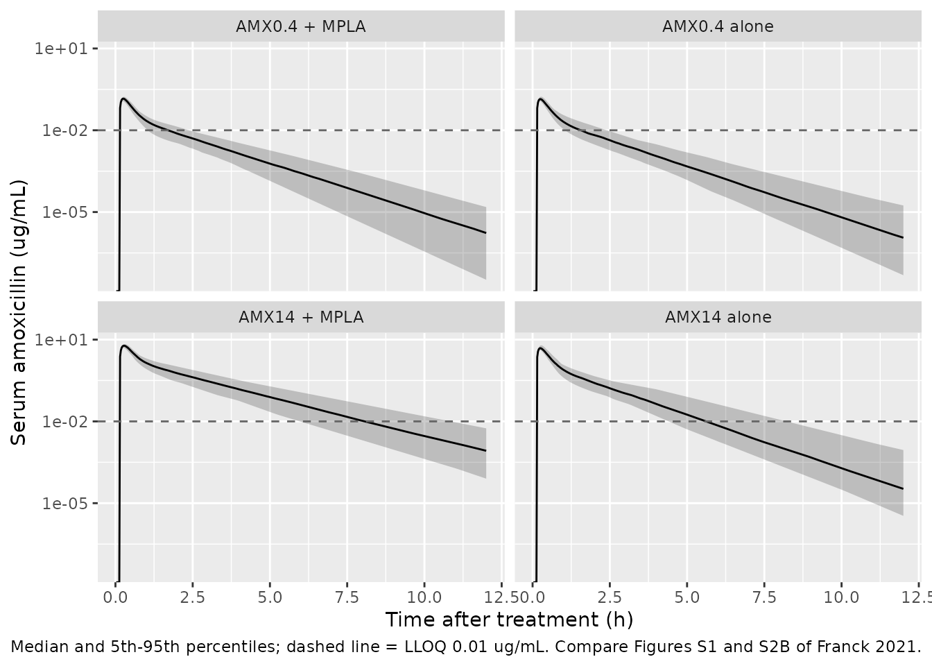

MPLA-dose interaction on clearance

The Results give the MPLA-coadministration clearance as 73.3 mL/h at 14 mg/kg (-40.9%) and 123 mL/h at 0.4 mg/kg (-1.17%). The typical-value model gives these values exactly, which pins the dose unit to ug per 25 g mouse.

first_ids <- (seq_len(nrow(pk_arms)) - 1L) * n_per_arm + 1L
pk_typ_events <- pk_events |> dplyr::filter(id %in% first_ids)
pk_typ <- rxode2::rxSolve(
  rxode2::zeroRe(readModelDb("Franck_2021_amoxicillin_mouse")),
  events = pk_typ_events, keep = "arm", returnType = "data.frame",
  atol = 1e-12, rtol = 1e-10
)
#> ℹ parameter labels from comments will be replaced by 'label()'
#> ℹ omega/sigma items treated as zero: 'etalcl', 'etalq'
#> Warning: multi-subject simulation without without 'omega'
cl_tab <- pk_typ |>
  dplyr::distinct(arm, cl) |>
  dplyr::mutate(pct_vs_mono = 100 * (cl / 124 - 1))
knitr::kable(cl_tab, digits = c(0, 2, 2), caption = "Typical CL/F by arm (mL/h).")

Typical CL/F by arm (mL/h).
arm	cl	pct_vs_mono
AMX0.4 alone	124.00	0.00
AMX0.4 + MPLA	122.55	-1.17
AMX14 alone	124.00	0.00
AMX14 + MPLA	73.25	-40.93


cl_of <- function(a) {
  v <- cl_tab$cl[cl_tab$arm == a]
  stopifnot(length(v) == 1L)
  v
}
stopifnot(
  abs(cl_of("AMX14 + MPLA") - 73.3) < 0.1,
  abs(cl_of("AMX0.4 + MPLA") - 123) < 0.5,
  abs(100 * (1 - cl_of("AMX14 + MPLA") / 124) - 40.9) < 0.1,
  abs(100 * (1 - cl_of("AMX0.4 + MPLA") / 124) - 1.17) < 0.01,
  abs(cl_of("AMX14 alone") - 124) < 1e-8
)

PKNCA

Noncompartmental analysis of the typical-value profiles (a fine grid to 12 h, then out to 24 h so the terminal phase is resolved). The paper reports no NCA table. The reference AUC below is Dose / CL computed from the clearances the paper states (124, 73.3 and 123 mL/h; F = 1). It tests the whole dose, unit and clearance chain.

nca_events <- pk_typ_events |>
  dplyr::filter(evid == 1L | time == 0) |>
  dplyr::bind_rows(
    tidyr::expand_grid(
      id = unique(pk_typ_events$id),
      time = sort(unique(c(pk_times, seq(12.5, 24, by = 0.5))))
    ) |>
      dplyr::mutate(evid = 0L, amt = 0, cmt = "central")
  ) |>
  dplyr::group_by(id) |>
  tidyr::fill(arm, DOSE_AMOXICILLIN_UG, CONMED_MPLA, .direction = "downup") |>
  dplyr::ungroup() |>
  dplyr::distinct(id, time, evid, .keep_all = TRUE) |>
  dplyr::arrange(id, time, dplyr::desc(evid))

nca_sim <- rxode2::rxSolve(
  rxode2::zeroRe(readModelDb("Franck_2021_amoxicillin_mouse")),
  events = nca_events, keep = "arm", returnType = "data.frame",
  atol = 1e-14, rtol = 1e-12
)
#> ℹ parameter labels from comments will be replaced by 'label()'
#> ℹ omega/sigma items treated as zero: 'etalcl', 'etalq'
#> Warning: multi-subject simulation without without 'omega'
stopifnot(all(nca_sim$Cc >= -1e-6 * max(nca_sim$Cc)))

conc_df <- nca_sim |>
  dplyr::filter(!is.na(Cc)) |>
  dplyr::mutate(Cc = pmax(Cc, 0), treatment = arm) |>
  dplyr::select(id, time, Cc, treatment)
conc_df <- dplyr::bind_rows(
  conc_df,
  conc_df |> dplyr::distinct(id, treatment) |> dplyr::mutate(time = 0, Cc = 0)
) |>
  dplyr::distinct(id, treatment, time, .keep_all = TRUE) |>
  dplyr::arrange(id, treatment, time)

dose_df <- nca_events |>
  dplyr::filter(evid == 1L) |>
  dplyr::transmute(id, time, amt, treatment = arm)

conc_obj <- PKNCA::PKNCAconc(conc_df, Cc ~ time | treatment + id)
dose_obj <- PKNCA::PKNCAdose(dose_df, amt ~ time | treatment + id)
intervals <- data.frame(
  start = 0, end = Inf,
  cmax = TRUE, tmax = TRUE, aucinf.obs = TRUE, half.life = TRUE
)
nca_res <- PKNCA::pk.nca(PKNCA::PKNCAdata(conc_obj, dose_obj, intervals = intervals))

published <- tibble::tribble(
  ~treatment,       ~aucinf.obs,
  "AMX0.4 alone",   10 / 124,
  "AMX0.4 + MPLA",  10 / 123,
  "AMX14 alone",    350 / 124,
  "AMX14 + MPLA",   350 / 73.3
)
cmp <- nlmixr2lib::ncaComparisonTable(
  simulated = nca_res,
  reference = published,
  by = "treatment",
  units = c(cmax = "ug/mL", tmax = "h", aucinf.obs = "h*ug/mL", half.life = "h"),
  tolerance_pct = 20
)
knitr::kable(
  cmp,
  caption = "Typical-value NCA. Reference AUC = dose / published CL (F = 1). * differs from reference by >20%."
)

Typical-value NCA. Reference AUC = dose / published CL (F = 1). * differs from reference by >20%.
NCA parameter	treatment	Reference	Simulated	% diff
AUC0-∞ (obs) (h*ug/mL)	AMX0.4 alone	0.0806	0.0805	-0.2%
AUC0-∞ (obs) (h*ug/mL)	AMX0.4 + MPLA	0.0813	0.0814	+0.1%
AUC0-∞ (obs) (h*ug/mL)	AMX14 alone	2.82	2.82	-0.2%
AUC0-∞ (obs) (h*ug/mL)	AMX14 + MPLA	4.77	4.77	-0.1%


auc_chk <- as.data.frame(nca_res) |>
  dplyr::filter(PPTESTCD == "aucinf.obs") |>
  dplyr::left_join(published, by = "treatment")
stopifnot(nrow(auc_chk) == 4L)
# Deterministic: both sides use the same typical parameters, so the only
# difference is the trapezoidal/extrapolation error of the NCA.
stopifnot(all(abs(auc_chk$PPORRES / auc_chk$aucinf.obs - 1) < 0.02))

PK/PD and survival model

Simulation design

Model time zero is the time of infection. Treatment is given at 12 h: an oral AMX dose into depot and, for MPLA arms, CONMED_MPLA switching from 0 to 1. The PD and survival parameters carry no interindividual variability (one observation per mouse), so each arm is a single typical-value solve. The 90% prediction band for the log10 CFU plots is the typical value +/- 1.645 times the additive residual SD.

pd_arms <- tibble::tribble(
  ~amx_mgkg, ~mpla,
  0, 0L,
  0.2, 0L,
  0.4, 0L,
  1.2, 0L,
  0, 1L,
  0.2, 1L,
  0.4, 1L,
  1.2, 1L
) |>
  dplyr::mutate(
    arm = dplyr::case_when(
      amx_mgkg == 0 & mpla == 0L ~ "Untreated",
      amx_mgkg == 0 ~ "MPLA",
      mpla == 0L ~ paste0("AMX", amx_mgkg),
      TRUE ~ paste0("AMX", amx_mgkg, " + MPLA")
    ),
    arm = factor(arm, levels = arm),
    dose_ug = amx_mgkg * bw_g
  )
t_treat <- 12
pd_times <- sort(unique(c(seq(0, 48, by = 0.25), seq(49, 336, by = 1))))

make_pd_arm <- function(k) {
  a <- pd_arms[k, ]
  obs_rows <- data.frame(
    time = pd_times, evid = 0L, amt = 0, cmt = NA_character_, dvid = 1L
  )
  dose_rows <- if (a$dose_ug > 0) {
    data.frame(time = t_treat, evid = 1L, amt = a$dose_ug, cmt = "depot", dvid = NA_integer_)
  } else {
    NULL
  }
  dplyr::bind_rows(dose_rows, obs_rows) |>
    dplyr::mutate(
      id = k,
      arm = as.character(a$arm),
      DOSE_AMOXICILLIN_UG = a$dose_ug,
      CONMED_MPLA = ifelse(time >= t_treat, a$mpla, 0L)
    ) |>
    dplyr::arrange(time, dplyr::desc(evid))
}
pd_events <- dplyr::bind_rows(lapply(seq_len(nrow(pd_arms)), make_pd_arm)) |>
  dplyr::relocate(id, time, evid, amt, cmt, dvid)

pd_sim <- rxode2::rxSolve(
  rxode2::zeroRe(readModelDb("Franck_2021_amoxicillin_mpla_mouse")),
  events = pd_events, keep = "arm", returnType = "data.frame",
  atol = 1e-10, rtol = 1e-8, maxsteps = 1e6
) |>
  dplyr::mutate(
    arm = factor(arm, levels = levels(pd_arms$arm)),
    time_after_treatment = time - t_treat
  )
#> Warning: No omega parameters in the model
#> Warning: multi-subject simulation without without 'omega'
stopifnot(dplyr::n_distinct(pd_sim$id) == nrow(pd_arms))

Figure 2A: lung bacterial burden

pd_sim |>
  dplyr::filter(time <= 48) |>
  ggplot(aes(time_after_treatment, log_cfu_lung)) +
  geom_ribbon(
    aes(
      ymin = log_cfu_lung - 1.645 * 1.12,
      ymax = log_cfu_lung + 1.645 * 1.12
    ),
    alpha = 0.2
  ) +
  geom_line() +
  facet_wrap(~arm, ncol = 4) +
  labs(
    x = "Time after treatment (h)", y = "log10 CFU / lung",
    caption = "Typical value and 90% prediction band. Replicates Figure 2A of Franck 2021."
  )

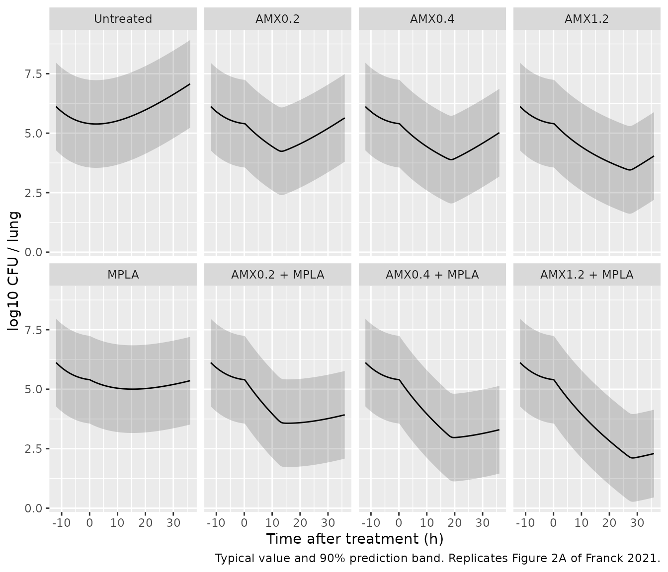
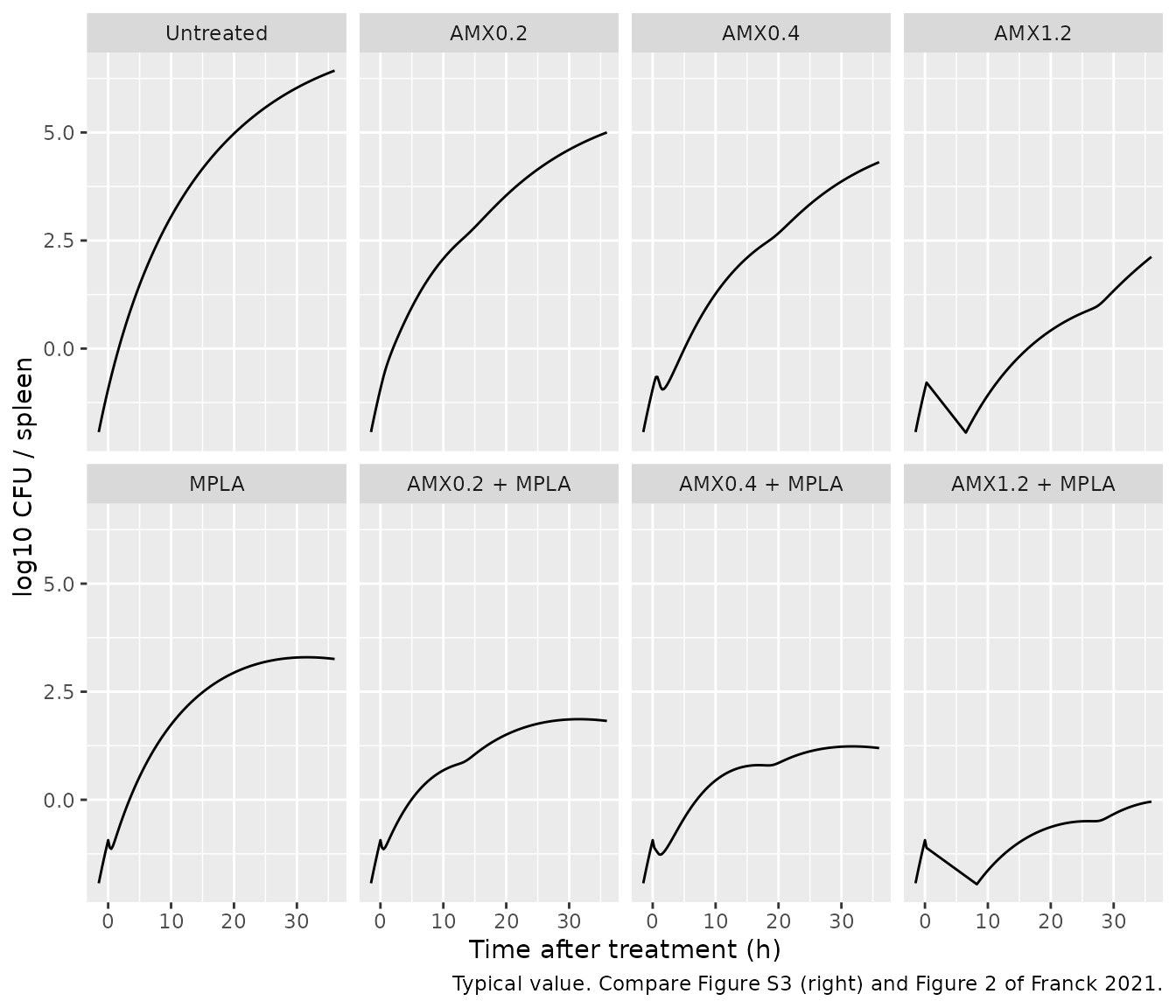
Figure S3: spleen bacterial burden

Bacteria first reach the spleen a few hours after treatment. Before that the spleen burden is effectively zero, so the plot starts where the burden exceeds 1 CFU.

pd_sim |>
  dplyr::filter(time <= 48, time_after_treatment >= -12, is.finite(log_cfu_spleen)) |>
  dplyr::filter(log_cfu_spleen > -2) |>
  ggplot(aes(time_after_treatment, log_cfu_spleen)) +
  geom_line() +
  facet_wrap(~arm, ncol = 4) +
  labs(
    x = "Time after treatment (h)", y = "log10 CFU / spleen",
    caption = "Typical value. Compare Figure S3 (right) and Figure 2 of Franck 2021."
  )

Published lung reductions at 36 h after treatment

The Results state that, compared with natural growth 36 h after treatment, AMX 1.2 mg/kg reduced the model-predicted lung burden by 3.03 log10 CFU, MPLA by 1.71 and the combination by 4.77.

lung36 <- pd_sim |>
  dplyr::filter(time_after_treatment == 36) |>
  dplyr::select(arm, log_cfu_lung)
untreated36 <- lung36$log_cfu_lung[lung36$arm == "Untreated"]
lung_cmp <- lung36 |>
  dplyr::mutate(reduction = untreated36 - log_cfu_lung) |>
  dplyr::left_join(
    tibble::tribble(
      ~arm, ~published,
      "AMX1.2", 3.03,
      "MPLA", 1.71,
      "AMX1.2 + MPLA", 4.77
    ) |>
      dplyr::mutate(arm = factor(arm, levels = levels(pd_arms$arm))),
    by = "arm"
  )
lung_cmp |>
  dplyr::rename(
    "Arm" = arm,
    "log10 CFU/lung at 36 h" = log_cfu_lung,
    "Reduction vs untreated (simulated)" = reduction,
    "Reduction vs untreated (published)" = published
  ) |>
  knitr::kable(digits = 2)

Arm	log10 CFU/lung at 36 h	Reduction vs untreated (simulated)	Reduction vs untreated (published)
Untreated	7.07	0.00	NA
AMX0.2	5.64	1.43	NA
AMX0.4	5.02	2.05	NA
AMX1.2	4.04	3.03	3.03
MPLA	5.36	1.71	1.71
AMX0.2 + MPLA	3.92	3.15	NA
AMX0.4 + MPLA	3.30	3.77	NA
AMX1.2 + MPLA	2.30	4.77	4.77


red_of <- function(a) lung_cmp$reduction[lung_cmp$arm == a]
# Deterministic typical-value solve against values printed to 2 decimals.
stopifnot(
  abs(red_of("AMX1.2") - 3.03) < 0.02,
  abs(red_of("MPLA") - 1.71) < 0.02,
  abs(red_of("AMX1.2 + MPLA") - 4.77) < 0.02
)

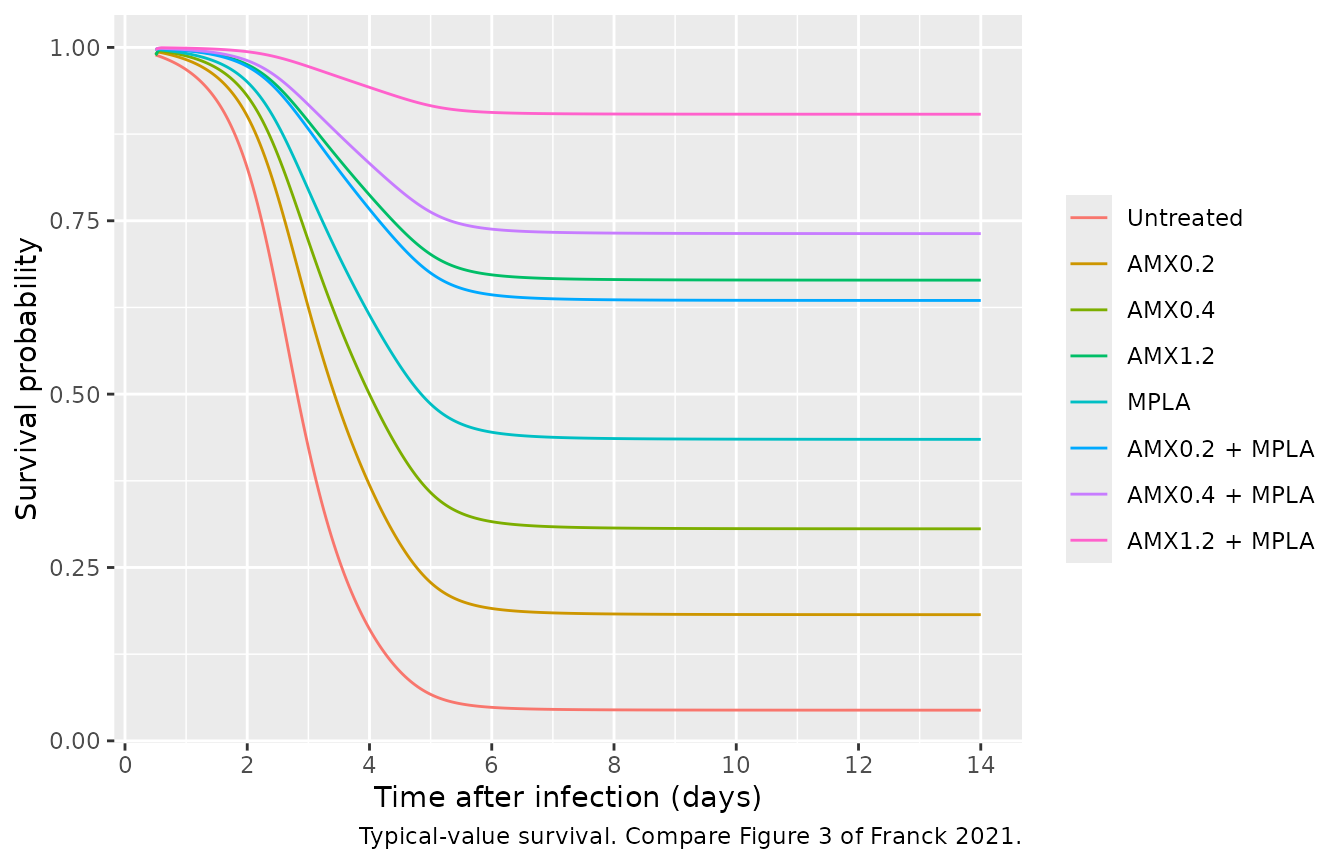
Figure 3: survival

pd_sim |>
  dplyr::filter(time >= t_treat) |>
  ggplot(aes(time / 24, sur, colour = arm)) +
  geom_line() +
  scale_x_continuous(breaks = seq(0, 14, by = 2)) +
  labs(
    x = "Time after infection (days)", y = "Survival probability", colour = NULL,
    caption = "Typical-value survival. Compare Figure 3 of Franck 2021."
  )

Published survival results

The Results report 14-day survival of 66.7% with AMX 1.2 mg/kg alone and 90.3% with AMX 1.2 mg/kg + MPLA, a 3.71-fold higher overall hazard in untreated than in MPLA-treated mice, and a 4.00-fold lower hazard when MPLA is added to AMX 1.2 mg/kg. The time above the MIC is taken at the end of the simulation.

end14 <- pd_sim |>
  dplyr::filter(time == 336) |>
  dplyr::select(arm, t_above_mic, cumhaz, sur)
knitr::kable(
  end14 |>
    dplyr::rename(
      "Arm" = arm,
      "T>MIC (h)" = t_above_mic,
      "Baseline cumulative hazard" = cumhaz,
      "Survival at 14 days" = sur
    ),
  digits = 3
)

Arm	T>MIC (h)	Baseline cumulative hazard	Survival at 14 days
Untreated	0.000	3.118	0.044
AMX0.2	0.653	3.118	0.182
AMX0.4	1.045	3.118	0.306
AMX1.2	2.194	3.118	0.664
MPLA	0.000	3.118	0.435
AMX0.2 + MPLA	0.655	3.118	0.635
AMX0.4 + MPLA	1.058	3.118	0.731
AMX1.2 + MPLA	2.275	3.118	0.904


val <- function(col, a) end14[[col]][end14$arm == a]
hr_mpla_alone <- exp(-(-1.32))
hr_amx12_mpla <- exp(-(-0.926 * (val("t_above_mic", "AMX1.2 + MPLA") -
  val("t_above_mic", "AMX1.2")) - 1.32))
surv_cmp <- tibble::tribble(
  ~quantity, ~simulated, ~published,
  "Survival at 14 d, AMX1.2", val("sur", "AMX1.2"), 0.667,
  "Survival at 14 d, AMX1.2 + MPLA", val("sur", "AMX1.2 + MPLA"), 0.903,
  "Hazard ratio untreated / MPLA", hr_mpla_alone, 3.71,
  "Hazard ratio AMX1.2 / AMX1.2 + MPLA", hr_amx12_mpla, 4.00
)
knitr::kable(surv_cmp, digits = 3)

quantity	simulated	published
Survival at 14 d, AMX1.2	0.664	0.667
Survival at 14 d, AMX1.2 + MPLA	0.904	0.903
Hazard ratio untreated / MPLA	3.743	3.710
Hazard ratio AMX1.2 / AMX1.2 + MPLA	4.036	4.000


stopifnot(
  abs(val("sur", "AMX1.2") - 0.667) < 0.01,
  abs(val("sur", "AMX1.2 + MPLA") - 0.903) < 0.01,
  abs(hr_mpla_alone / 3.71 - 1) < 0.02,
  abs(hr_amx12_mpla / 4.00 - 1) < 0.02
)

The Results also give the T>MIC needed for more than 95% survival: 4.48 h with AMX alone and 3.25 h with MPLA. Solving S(14 d) = 0.95 with the Table 2 estimates gives the values below. They are close for AMX alone and about 0.24 h lower with MPLA. The printed thresholds are reported, not used to change the model.

h0_14d <- val("cumhaz", "Untreated")
t_thr <- c(
  "AMX alone" = log(-log(0.95) / h0_14d) / -0.926,
  "AMX + MPLA" = (log(-log(0.95) / h0_14d) + 1.32) / -0.926
)
knitr::kable(
  data.frame(
    Regimen = names(t_thr),
    "T>MIC for 95% survival, from Table 2 (h)" = unname(t_thr),
    "Printed in Results (h)" = c(4.48, 3.25),
    check.names = FALSE
  ),
  digits = 2
)

Regimen	T>MIC for 95% survival, from Table 2 (h)	Printed in Results (h)
AMX alone	4.44	4.48
AMX + MPLA	3.01	3.25

Assumptions and deviations

Dose units. The paper gives doses in mg/kg and the MPLA clearance interaction slope in mL/h/ug. The clearances printed in the Results (73.3 mL/h at 14 mg/kg and 123 mL/h at 0.4 mg/kg with MPLA) are reproduced exactly when the dose is the mg/kg dose times a 25 g body weight, in ug. The models therefore take the dose as an absolute amount in ug per mouse (DOSE_AMOXICILLIN_UG), and a 25 g mouse is used throughout.
MPLA onset. CONMED_MPLA is time-varying: 0 before treatment and 1 from the 12 h treatment time onward. Switching MPLA on from the time of infection gives a 2.28 rather than the published 1.71 log10 CFU/lung reduction at 36 h.
Lung-to-spleen transit. Supplementary Equation 3 uses the Savic analytical transit input with the Stirling approximation for n!. The implementation applies that input kernel to the current lung burden (in place of a dose amount), does not deplete the lung, and has no spleen outflow other than drug and MPLA killing. A plain chain of transit compartments did not reproduce the spleen time course.
Spleen AMX kill constant. Table 1 gives kAMX as 13.7 with unit log10(h-1). The model uses kAMX = 10^13.7, applied to the spleen effect-compartment concentration raised to H_spleen = 5.06.
Time above MIC. The text calls the survival covariate %T>MIC but gives the thresholds in hours, and the published 14-day survival values reproduce when it is in hours. The model accumulates the time (h) that the serum concentration is at or above the MIC of 0.016 ug/mL. The hazard uses the running value. After a single dose it reaches its final value within a few hours of treatment, while the baseline hazard is still negligible.
Hazard time origin. Figure S4 plots the hazard against time after treatment, while the survival study counts days after infection. The model uses time after infection. Moving the origin by 12 h changes 14-day survival by less than 0.001, because the surge peaks at 89 h.
EC50. Table 1 gives 0.00109 ug/mL, within its bootstrap interval (0.000134-0.00146). The Results text gives 0.0109. The table value is used.
Mean transit time. Table 1 gives 40.8 h. The Supplementary Section S3 text gives 42.0 h. The table value is used.
Figure S3, AMX 0.4 mg/kg + MPLA (spleen). The figure shows the spleen cleared of bacteria. The model gives about 1.2 log10 CFU/spleen at 36 h after treatment, consistent with Figure 2B.
Survival thresholds. From the Table 2 estimates, the T>MIC giving 95% survival at 14 days is 4.44 h (AMX alone) and 3.01 h (with MPLA), against the printed 4.48 h and 3.25 h (see above).
Figure S4 axis. The hazard axis is labelled per day, but the plotted values match the Table 2 surge amplitude in 1/h.
Survival residual error. The source has no residual error for the survival probability. addSd_sur is a fixed placeholder (0.001) so that the sur output has an error model for simulation. It is not from the source.
PK in the PK/PD model. Following Table 1 footnote *, the PK parameters are fixed at the PK submodel typical values without IIV. H_lung = 20 and the initial lung burden (6.12 log10 CFU at infection) are fixed as in Table 1.
PKNCA reference values. The paper has no NCA table. The reference AUCs are dose / CL from the clearances printed in the paper.