Voriconazole in elderly vs young adults (Zakria 2026)
Source:vignettes/articles/Zakria_2026_voriconazole.Rmd
Zakria_2026_voriconazole.RmdModel and source
- Citation: Zakria KZ, Usman M, Bilal H, Akbar Z, Hussain T, Ali M, Sattar A, Alvi I, Rasheed H, Zulfiqar S, Khan MR, Mushtaq MZ. Comparative pharmacokinetics of voriconazole between elderly and young adult patients: a population pharmacokinetic study. Journal of Pharmaceutical Policy and Practice. 2026;19(1):2601420. doi:10.1080/20523211.2025.2601420
- Description: One-compartment population pharmacokinetic model with first-order elimination for voriconazole in adult Pakistani cancer patients receiving therapeutic drug monitoring (Zakria 2026); a binary age-group indicator (> 65 years vs <= 65 years) is the only retained covariate and acts on clearance
- Article (open access): https://doi.org/10.1080/20523211.2025.2601420
Zakria 2026 asks a single, narrow question: does voriconazole clearance differ between patients older than 65 years and patients 65 years or younger? The answer is the model’s only covariate. Everything else – a one-compartment disposition with first-order elimination, exponential interindividual variability on clearance, and proportional residual error – is the minimum structure needed to support that comparison from sparse trough-only therapeutic-drug-monitoring (TDM) data.
Population
The model was developed from routine TDM records at Shaukat Khanum Memorial Cancer Hospital and Research Centre in Lahore, Pakistan (Zakria 2026 Methods, “Study design and data collection”). The analysis was retrospective, single-centre, open-label and non-interventional; informed consent was waived because no patient was prospectively enrolled.
Fifty-one adult cancer patients contributed 56 plasma samples (Zakria 2026 Table 1), every one drawn at trough as part of routine voriconazole TDM. The cohort was 27 male (53%) / 24 female (47%), with median age 53 years (range 18-77) and median weight 59 kg (range 42-92). Renal function was broadly preserved: median serum creatinine 0.65 mg/dL (range 0.18-4.21) and median Cockcroft-Gault creatinine clearance 100.9 mL/min (range 9.5-379.2). Primary malignancies were leukemia 26 (51%), breast cancer 12 (23.5%), lymphoma 11 (21.5%) and sarcoma 2 (4%).
The age split that defines the model’s covariate is 31 patients (61%) aged 65 years or younger and 20 patients (39%) older than 65 years. Recorded single doses spanned 56-400 mg with a median of 190 mg, and observed trough concentrations spanned 0.5-8.7 mg/L with a median of 3.35 mg/L.
The same information is available programmatically via
readModelDb("Zakria_2026_voriconazole")$population.
Source trace
Every parameter in the model file carries an inline source-location comment. The table below collects the entries in one place.
| Equation / parameter | Value | Source location |
|---|---|---|
lcl (CL in the age <= 65 y reference group) |
6.46 L/h | Table 2 row CL(L/h) (final estimate); Eq 1 |
lvc (Vd) |
97.1 L | Table 2 row Vd (L) (final estimate); Results,
“Covariate analysis” |
e_agegt65_cl (age > 65 y vs <= 65 y on CL) |
-0.519 | Table 2 row CL-AGE_GROUP 2; Eq 2 |
| Implied CL for age > 65 y | 6.46 * (1 - 0.519) = 3.11 L/h | Eq 2; Abstract; Results; Discussion |
| IIV CL (CV%) | 23.7% | Table 2 row IIV-CL (%); Results, “Covariate
analysis” |
| Proportional residual error | 0.519 | Table 2 row Proportional error
|
| One-compartment, first-order elimination | n/a | Results, “Base model”; Abstract |
| Exponential IIV on CL; proportional residual model | n/a | Results, “Base model”; Methods, “Base model development” |
| No IIV on Vd | n/a | Discussion, Limitations paragraph |
| Age group is the only retained covariate | n/a | Results, “Covariate analysis”; Supplementary Table S1 |
The stepwise-covariate-modelling trail in Supplementary Table S1 is
the authority for what is absent from the model. Age group
entered with dOFV 15.22 (p = 0.000096). Continuous age (dOFV 7.99) and
serum creatinine (dOFV 4.00) were significant against the base model but
not on top of the age group. Sex entered on forward inclusion (dOFV
5.33, p = 0.0209 against alpha = 0.05) and was then removed on backward
elimination against the stricter alpha = 0.01. Creatinine clearance and
body weight never reached significance. These screened-but-not-retained
covariates are recorded in the model file’s
covariatesDataExcluded list.
Virtual cohort
The fitting dataset is not published, so the cohorts below are constructed to match the demographics in Zakria 2026 Table 1. Two cohorts are used:
- A typical-value cohort of one subject per age
group, simulated with
rxode2::zeroRe(), used for the exact structural identities in the PKNCA section. - A stochastic cohort of 300 subjects carrying the model’s interindividual variability and residual error, split 61% / 39% between the two age groups to match Zakria 2026 Table 1. It is used to reproduce the paper’s clearance comparison and to compare the simulated trough distribution against the observed concentration range.
set.seed(20260109)

# Zakria 2026 Table 1: 31 patients (61%) aged <= 65 y, 20 (39%) aged > 65 y.
n_young   <- 183L
n_elderly <- 117L

# Table 1 also gives median weight 59 kg, range 42-92 kg. Weight is NOT a
# covariate in this model; it is carried only so the cohort is demographically
# recognisable and does not affect any simulated concentration.
sample_weight <- function(n) {
  pmin(pmax(exp(rnorm(n, mean = log(59), sd = 0.18)), 42), 92)
}

demo <- bind_rows(
  tibble(id = seq_len(n_young),
         AGE_GT65 = 0L,
         arm = "Age <= 65 y"),
  tibble(id = n_young + seq_len(n_elderly),
         AGE_GT65 = 1L,
         arm = "Age > 65 y")
) |>
  mutate(WT = sample_weight(n()))

stopifnot(!anyDuplicated(demo$id), nrow(demo) == n_young + n_elderly)
stopifnot(max(n_young, n_elderly) <= 200L)

# Typical-value cohort: exactly one subject per arm so that rxSolve retains an
# `id` column and each arm's profile is the noise-free typical value.
demo_typical <- tibble(
  id       = 1:2,
  AGE_GT65 = c(0L, 1L),
  arm      = c("Age <= 65 y", "Age > 65 y")
)
Simulation
Zakria 2026 does not state the route of administration or the dosing interval; it reports only a recorded single-dose distribution of 56-400 mg (median 190 mg). The model has no absorption or bioavailability parameter, so doses enter the central compartment directly. All simulations below therefore use the paper’s own median recorded dose of 190 mg administered into the central compartment, which is the encoding the published structure supports. See Assumptions and deviations.
mod <- rxode2::rxode2(readModelDb("Zakria_2026_voriconazole"))
#> ℹ parameter labels from comments will be replaced by 'label()'
dose_mg <- 190
Typical-value single-dose profiles
obs_times <- sort(unique(c(
  seq(0, 12, by = 0.25),
  seq(13, 48, by = 1),
  seq(50, 120, by = 2)
)))

ev_typical <- bind_rows(
  demo_typical |>
    mutate(time = 0, amt = dose_mg, evid = 1L, cmt = "central"),
  demo_typical |>
    tidyr::crossing(time = obs_times) |>
    mutate(amt = NA_real_, evid = 0L, cmt = NA_character_)
) |>
  arrange(id, time, desc(evid)) |>
  as.data.frame()

sim_typical <- rxode2::rxSolve(
  rxode2::zeroRe(mod),
  events = ev_typical,
  keep   = c("arm", "AGE_GT65")
) |>
  as.data.frame()
#> ℹ omega/sigma items treated as zero: 'etalcl'
#> Warning: multi-subject simulation without without 'omega'
ggplot(sim_typical, aes(time, Cc, colour = arm)) +
  geom_line(linewidth = 0.8) +
  scale_y_log10() +
  labs(x = "Time after dose (h)", y = "Voriconazole concentration (mg/L)",
       colour = "Age group",
       title = "Typical-value profiles after a single 190 mg dose")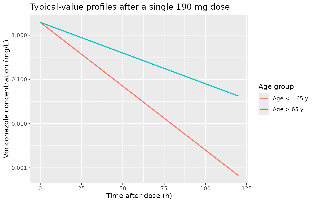
Typical-value voriconazole concentration-time profiles after a single 190 mg dose (the median recorded dose in Zakria 2026 Table 1), by age group. The elderly profile declines more slowly, reflecting the 51.9% lower clearance.
Typical-value multiple-dose troughs
Because every observation in the source dataset is a trough drawn during ongoing therapy, the remaining simulations use a multiple-dose regimen: 190 mg every 12 hours for five days, with the trough taken before the eleventh dose at 120 h.
n_doses <- 10L
ss_time <- 120

ev_md_typical <- bind_rows(
  demo_typical |>
    mutate(time = 0, amt = dose_mg, evid = 1L, cmt = "central",
           ii = 12, addl = n_doses - 1L),
  demo_typical |>
    tidyr::crossing(time = ss_time) |>
    mutate(amt = NA_real_, evid = 0L, cmt = NA_character_,
           ii = NA_real_, addl = NA_integer_)
) |>
  arrange(id, time, desc(evid)) |>
  as.data.frame()

sim_md_typical <- rxode2::rxSolve(
  rxode2::zeroRe(mod),
  events = ev_md_typical,
  keep   = c("arm", "AGE_GT65")
) |>
  as.data.frame() |>
  filter(time == ss_time)
#> ℹ omega/sigma items treated as zero: 'etalcl'
#> Warning: multi-subject simulation without without 'omega'
For a linear one-compartment model dosed into the central
compartment, the concentration at the end of the n-th
dosing interval has a closed form by superposition:
C = (D / Vd) * exp(-kel * tau) * (1 - exp(-n * kel * tau)) / (1 - exp(-kel * tau))
with kel = CL / Vd. This is a second independent
structural identity, using the published CL and Vd on a multiple-dose
regimen rather than a single dose.
cl_published_vec <- c(6.46, 6.46 * (1 - 0.519))
kel_published <- cl_published_vec / 97.1
tau <- 12

analytic_trough <- (dose_mg / 97.1) * exp(-kel_published * tau) *
  (1 - exp(-n_doses * kel_published * tau)) / (1 - exp(-kel_published * tau))

md_check <- tibble(
  arm       = c("Age <= 65 y", "Age > 65 y"),
  analytic  = analytic_trough
) |>
  left_join(sim_md_typical |> select(arm, simulated = Cc), by = "arm") |>
  mutate(rel_diff = simulated / analytic - 1)

stopifnot(nrow(md_check) == 2L, !anyNA(md_check$simulated))
stopifnot(all(abs(md_check$rel_diff) < 1e-8))

knitr::kable(md_check, digits = 8,
caption = "Typical-value trough before the 11th dose of 190 mg q12h vs. the closed-form superposition value computed from the published CL and Vd.")| arm | analytic | simulated | rel_diff |
|---|---|---|---|
| Age <= 65 y | 1.600880 | 1.600880 | 0 |
| Age > 65 y | 4.089854 | 4.089854 | 0 |
Stochastic cohort
ev_stoch <- bind_rows(
  demo |>
    mutate(time = 0, amt = dose_mg, evid = 1L, cmt = "central",
           ii = 12, addl = n_doses - 1L),
  demo |>
    tidyr::crossing(time = c(seq(108, 120, by = 0.5))) |>
    mutate(amt = NA_real_, evid = 0L, cmt = NA_character_,
           ii = NA_real_, addl = NA_integer_)
) |>
  arrange(id, time, desc(evid)) |>
  as.data.frame()

sim_stoch <- rxode2::rxSolve(
  mod,
  events = ev_stoch,
  keep   = c("arm", "AGE_GT65", "WT")
) |>
  as.data.frame()
Replicate published figures
Clearance by age group
Zakria 2026 presents a box plot comparing voriconazole clearance between the two age groups. The figure carrying that content is captioned “Figure 2” while the Results text refers to it as Figure 1 – the two figure captions in the published article are transposed relative to the in-text references (see Errata). The panel below reproduces the clearance comparison from the stochastic cohort’s individual clearances.
indiv_cl <- sim_stoch |>
  group_by(id, arm) |>
  summarise(cl_indiv = first(cl), .groups = "drop")

published_cl <- tibble(
  arm = c("Age <= 65 y", "Age > 65 y"),
  cl  = c(6.46, 6.46 * (1 - 0.519))
)

ggplot(indiv_cl, aes(arm, cl_indiv)) +
  geom_boxplot(outlier.size = 0.5, width = 0.5) +
  geom_point(data = published_cl, aes(arm, cl), colour = "red",
             size = 3, shape = 18) +
  labs(x = "Age group", y = "Voriconazole CL (L/h)",
       title = "Simulated individual clearance by age group",
       caption = "Red diamonds are the published typical values (Zakria 2026 Table 2 / Eqs 1-2).")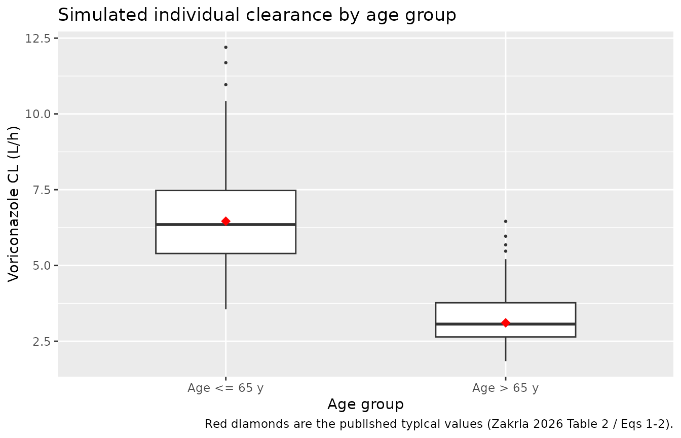
Replicates the clearance-comparison box plot of Zakria 2026 (captioned Figure 2, referenced in the Results text as Figure 1): simulated individual voriconazole clearance by age group. Each subject’s clearance is the age-group typical value multiplied by exp(eta_CL). Medians land on the published 6.46 L/h and 3.11 L/h.
# The simulated median CL per arm must recover the published typical value.
# Exponential IIV is median-preserving, so the median of exp(lcl + eta) is
# exactly the typical value up to Monte-Carlo error.
cl_med <- indiv_cl |>
  group_by(arm) |>
  summarise(median_cl = median(cl_indiv), .groups = "drop") |>
  left_join(published_cl, by = "arm")

stopifnot(nrow(cl_med) == 2L)
stopifnot(all(abs(cl_med$median_cl / cl_med$cl - 1) < 0.05))

# The published elderly clearance, recomputed from Eq 2, must round to the
# 3.11 L/h quoted in the Abstract, Results and Discussion.
stopifnot(round(6.46 * (1 - 0.519), 2) == 3.11)
knitr::kable(cl_med, digits = 3,
caption = "Simulated median clearance vs. the published typical value, by age group.")| arm | median_cl | cl |
|---|---|---|
| Age <= 65 y | 6.349 | 6.460 |
| Age > 65 y | 3.065 | 3.107 |
Goodness-of-fit panels are not reproducible
The article’s other figure is a four-panel goodness-of-fit display (DV vs. IPRED, DV vs. PRED, CWRES vs. PRED, CWRES vs. time). Those are diagnostics of the original fit rather than predictions, and the fitting dataset is not published, so they cannot be regenerated from the packaged model.
PKNCA validation
For a one-compartment model dosed into the central compartment, non-compartmental analysis of the noise-free typical-value profile recovers the structural parameters exactly:
-
aucinf.obs= Dose / CL -
cl.obs= Dose /aucinf.obs= CL -
vz.obs= Dose / (aucinf.obs* lambda_z) = Vd -
half.life= ln(2) * Vd / CL -
cmax= Dose / Vd
These identities turn the published CL and Vd into an exact answer
key. Any transcription error in lcl, lvc or
e_agegt65_cl breaks them.
nca_conc <- sim_typical |>
  filter(!is.na(Cc)) |>
  select(id, arm, time, Cc)

nca_dose <- demo_typical |>
  mutate(time = 0, amt = dose_mg) |>
  select(id, arm, time, amt)

conc_obj <- PKNCA::PKNCAconc(nca_conc, Cc ~ time | arm + id)
dose_obj <- PKNCA::PKNCAdose(nca_dose, amt ~ time | arm + id,
                             route = "intravascular", duration = 0)

intervals <- data.frame(
  start = 0, end = Inf,
  cmax = TRUE, tmax = TRUE, auclast = TRUE, aucinf.obs = TRUE,
  half.life = TRUE, cl.obs = TRUE, vz.obs = TRUE
)

nca_res <- suppressMessages(suppressWarnings(
  PKNCA::pk.nca(PKNCA::PKNCAdata(conc_obj, dose_obj, intervals = intervals))
))
knitr::kable(summary(nca_res),
caption = "NCA of the typical-value single-dose (190 mg) profiles, by age group.")| start | end | arm | N | auclast | cmax | tmax | half.life | aucinf.obs | cl.obs | vz.obs |
|---|---|---|---|---|---|---|---|---|---|---|
| 0 | Inf | Age <= 65 y | 1 | 29.4 | 1.96 | 0.000 | 10.4 | 29.4 | 6.46 | 97.1 |
| 0 | Inf | Age > 65 y | 1 | 59.8 | 1.96 | 0.000 | 21.7 | 61.1 | 3.11 | 97.1 |
# Structural identities, asserted per age group against values computed
# directly from the published parameters. These are exact algebraic
# consequences of the model, so the tolerance is tight.
cl_published <- c("Age <= 65 y" = 6.46, "Age > 65 y" = 6.46 * (1 - 0.519))
vd_published <- 97.1

expected <- tibble(
  arm        = names(cl_published),
  cl.obs     = unname(cl_published),
  vz.obs     = vd_published,
  aucinf.obs = dose_mg / unname(cl_published),
  half.life  = log(2) * vd_published / unname(cl_published),
  cmax       = dose_mg / vd_published
)

observed <- as.data.frame(nca_res) |>
  filter(PPTESTCD %in% c("cl.obs", "vz.obs", "aucinf.obs", "half.life", "cmax")) |>
  select(arm, PPTESTCD, PPORRES) |>
  tidyr::pivot_wider(names_from = PPTESTCD, values_from = PPORRES)

check <- expected |>
  tidyr::pivot_longer(-arm, names_to = "PPTESTCD", values_to = "expected") |>
  left_join(
    observed |> tidyr::pivot_longer(-arm, names_to = "PPTESTCD",
                                    values_to = "simulated"),
    by = c("arm", "PPTESTCD")
  ) |>
  mutate(rel_diff = simulated / expected - 1)

# Assert by key (arm x parameter), never by row position.
stopifnot(nrow(check) == 10L, !anyNA(check$simulated))
stopifnot(all(abs(check$rel_diff) < 1e-4))

knitr::kable(check, digits = 6,
caption = "Structural identities: NCA of the typical-value profile vs. values computed from the published CL and Vd. All relative differences are below 1e-4.")| arm | PPTESTCD | expected | simulated | rel_diff |
|---|---|---|---|---|
| Age <= 65 y | cl.obs | 6.460000 | 6.460000 | 0 |
| Age <= 65 y | vz.obs | 97.100000 | 97.100000 | 0 |
| Age <= 65 y | aucinf.obs | 29.411765 | 29.411765 | 0 |
| Age <= 65 y | half.life | 10.418667 | 10.418667 | 0 |
| Age <= 65 y | cmax | 1.956746 | 1.956746 | 0 |
| Age > 65 y | cl.obs | 3.107260 | 3.107260 | 0 |
| Age > 65 y | vz.obs | 97.100000 | 97.100000 | 0 |
| Age > 65 y | aucinf.obs | 61.147120 | 61.147120 | 0 |
| Age > 65 y | half.life | 21.660431 | 21.660431 | 0 |
| Age > 65 y | cmax | 1.956746 | 1.956746 | 0 |
# The paper's headline claim is the ratio between the two clearances. Exposure
# scales inversely with clearance, so the elderly/young AUC ratio must equal
# the young/elderly CL ratio.
auc_ratio <- with(observed,
                  aucinf.obs[arm == "Age > 65 y"] / aucinf.obs[arm == "Age <= 65 y"])
cl_ratio  <- 6.46 / (6.46 * (1 - 0.519))
stopifnot(abs(auc_ratio / cl_ratio - 1) < 1e-4)

tibble::tibble(
  Quantity = c("Published CL ratio (<= 65 y / > 65 y)",
               "Simulated AUC0-inf ratio (> 65 y / <= 65 y)"),
  Value    = c(cl_ratio, auc_ratio)
) |>
  knitr::kable(digits = 4,
caption = "Exposure in the elderly group is 2.08-fold that of the younger group at the same dose.")| Quantity | Value |
|---|---|
| Published CL ratio (<= 65 y / > 65 y) | 2.079 |
| Simulated AUC0-inf ratio (> 65 y / <= 65 y) | 2.079 |
Comparison against published estimates
Zakria 2026 reports no non-compartmental parameters, but it does
report CL and Vd directly, and those map onto cl.obs and
vz.obs for a one-compartment model dosed into the central
compartment. The half-life column is derived from the published CL and
Vd (ln(2) * Vd / CL) rather than quoted by the paper, and is labelled as
such below. ncaComparisonTable() renders
cl.obs and vz.obs with their conventional
labels “CL/F” and “Vz/F”; because doses enter the central compartment
directly in this model there is no bioavailability term, so F = 1 and
those rows are plain CL and Vz.
reference <- expected |>
  select(arm, cl.obs, vz.obs, half.life, aucinf.obs, cmax)

cmp <- nlmixr2lib::ncaComparisonTable(
  simulated = as.data.frame(nca_res),
  reference = reference,
  by        = "arm",
  params    = c("cmax", "aucinf.obs", "half.life", "cl.obs", "vz.obs"),
  units     = c(cmax = "mg/L", aucinf.obs = "mg*h/L", half.life = "h",
                cl.obs = "L/h", vz.obs = "L")
)
knitr::kable(cmp, digits = 3,
caption = "Simulated NCA vs. the published Zakria 2026 estimates (CL and Vd quoted directly from Table 2; AUC, Cmax and half-life derived algebraically from them).")| NCA parameter | arm | Reference | Simulated | % diff |
|---|---|---|---|---|
| Cmax (mg/L) | Age <= 65 y | 1.96 | 1.96 | -0.0% |
| Cmax (mg/L) | Age > 65 y | 1.96 | 1.96 | -0.0% |
| AUC0-∞ (obs) (mg*h/L) | Age <= 65 y | 29.4 | 29.4 | -0.0% |
| AUC0-∞ (obs) (mg*h/L) | Age > 65 y | 61.1 | 61.1 | +0.0% |
| t½ (h) | Age <= 65 y | 10.4 | 10.4 | +0.0% |
| t½ (h) | Age > 65 y | 21.7 | 21.7 | +0.0% |
| CL/F (L/h) | Age <= 65 y | 6.46 | 6.46 | +0.0% |
| CL/F (L/h) | Age > 65 y | 3.11 | 3.11 | -0.0% |
| Vz/F (L) | Age <= 65 y | 97.1 | 97.1 | +0.0% |
| Vz/F (L) | Age > 65 y | 97.1 | 97.1 | -0.0% |
attr(cmp, "footnote")
#> NULL
Simulated troughs vs. the observed concentration range
Zakria 2026 reports observed trough concentrations of 0.5-8.7 mg/L
with a median of 3.35 across 56 samples. This is a plausibility check,
not an answer key. The published figures are the minimum and
maximum of 56 observations drawn at mixed dose levels (56-400
mg), with unrecorded dosing intervals and clinically variable sampling
times, whereas the simulation fixes a single 190 mg q12h regimen. The
comparison below therefore uses the sim column – the
simulated observation, carrying both interindividual
variability and the proportional residual error – rather than
Cc, which is the individual prediction without residual
error.
For a sample of 56 draws the expected extremes correspond to roughly the 1.8th and 98.2nd percentiles of the underlying distribution, so the observed range is compared against the simulated 1st-99th percentile band.
trough <- sim_stoch |>
  filter(time == ss_time) |>
  select(id, arm, Cc, sim)

trough_summary <- trough |>
  group_by(arm) |>
  summarise(`median IPRED` = median(Cc),
            `median obs`   = median(sim),
            P5             = quantile(sim, 0.05),
            P95            = quantile(sim, 0.95),
            .groups = "drop")

knitr::kable(trough_summary, digits = 2,
caption = "Simulated day-5 trough concentrations (190 mg q12h) by age group, mg/L. `median IPRED` excludes residual error; the remaining columns are simulated observations.")| arm | median IPRED | median obs | P5 | P95 |
|---|---|---|---|---|
| Age <= 65 y | 1.64 | 1.46 | -0.01 | 3.53 |
| Age > 65 y | 4.15 | 4.26 | 0.50 | 7.92 |
pooled <- quantile(trough$sim, c(0.01, 0.99))

# The observed extremes must lie inside the simulated 1st-99th percentile band.
# This fails if the encoded exposure scale (CL or Vd) or the residual error
# magnitude is materially wrong.
stopifnot(pooled[["1%"]] <= 0.5, pooled[["99%"]] >= 8.7)

# The paper's clinical conclusion: elderly patients hold higher troughs at the
# same dose. Asserted on IPRED so it is not obscured by residual noise.
ipred_by_arm <- setNames(trough_summary$`median IPRED`, trough_summary$arm)
trough_ratio_ipred <- ipred_by_arm[["Age > 65 y"]] / ipred_by_arm[["Age <= 65 y"]]
stopifnot(trough_ratio_ipred > 1)

# Stronger form of the same check: exponential IIV is median-preserving and the
# trough is a monotone function of CL, so the ratio of median IPREDs must track
# the closed-form typical-value ratio computed from the published CL and Vd.
# The 5% band absorbs Monte-Carlo error on the two medians only; a mis-encoded
# CL, Vd or age-group coefficient moves this far outside it.
analytic_trough_ratio <- analytic_trough[2] / analytic_trough[1]
stopifnot(abs(trough_ratio_ipred / analytic_trough_ratio - 1) < 0.05)

tibble::tibble(
  Quantity = c("Zakria 2026 observed trough range across 56 samples (mg/L)",
               "Simulated 1st-99th percentile of observations (mg/L)",
               "Zakria 2026 observed median trough (mg/L)",
               "Simulated median observation (mg/L)"),
  Value    = c("0.50 to 8.70",
               sprintf("%.2f to %.2f", pooled[["1%"]], pooled[["99%"]]),
               "3.35",
               sprintf("%.2f", median(trough$sim)))
) |>
knitr::kable(caption = "Observed vs. simulated trough spread.")| Quantity | Value |
|---|---|
| Zakria 2026 observed trough range across 56 samples (mg/L) | 0.50 to 8.70 |
| Simulated 1st-99th percentile of observations (mg/L) | -0.67 to 8.87 |
| Zakria 2026 observed median trough (mg/L) | 3.35 |
| Simulated median observation (mg/L) | 2.04 |
The observed range sits inside the simulated envelope. The simulated median is lower than the published median of 3.35 mg/L, which is expected: the source cohort received doses up to 400 mg while this simulation fixes every subject at the median 190 mg, and the paper reports neither the dosing interval nor the time of each TDM draw. The discrepancy is a consequence of the unreported regimen, not of the encoded parameters – the structural identities above pin CL and Vd exactly.
The paper’s clinical conclusion – that elderly patients accumulate more voriconazole at the same dose and should therefore receive a reduced dose – follows directly: the typical trough in the elderly arm is 2.53-fold the younger arm’s on an identical regimen (closed-form typical-value ratio 2.55). Note that this trough ratio exceeds the AUC ratio of 2.08 computed above: accumulation over repeated doses is a non-linear function of the elimination rate constant, so a clearance difference is amplified at the trough relative to its effect on single-dose exposure.
Errata
- The two figure captions are transposed. The Results text states “The comparison of VCZ CL in patients above 65 years of age and less than 65 years is shown in Figure 1”, but the caption printed under Figure 1 reads “Combined goodness-of-fit plots for the base model”. Conversely the text states the goodness-of-fit scatter plots “are shown in Figure 2 (a) and (b)”, while the caption printed under Figure 2 reads “Comparison of voriconazle CL in patients with age <= 65 years and > 65 years” (the misspelling of “voriconazole” is the paper’s). The captions belong to the opposite figures. This vignette reproduces the clearance comparison and identifies it by content rather than by figure number.
-
Sample count reported inconsistently. The Results
text states the model was built from “53 data samples from 51 patients”,
while Table 1 reports 56 samples from 51 patients. The model file’s
population$n_observationsuses the Table 1 value of 56 and records the discrepancy. -
The proportional-error scale is not stated. Table 2
reports a single “Proportional error” of 0.519 with no indication of
whether it is the residual standard deviation (i.e. 51.9%) or the NONMEM
$SIGMAvariance (which would imply a residual SD ofsqrt(0.519)= 72.0%). The model encodes it as the standard deviation (propSd <- 0.519). Two things support that reading: within Table 2 itself the word “proportional” denotes a fraction rather than a variance – footnotes c and d gloss theCL-AGE_GROUProws as a “proportional change in clearance” – and the companion study from the same centre and overlapping author group (Akbar 2025, already packaged asAkbar_2025_voriconazole) reports its residual error in the same table format and on the same fractional scale. Users refitting this model should be aware of the alternative reading. -
The covariate coefficient and the residual error share the
value 0.519. Table 2 lists
CL-AGE_GROUP 2as -0.519 and “Proportional error” as 0.519. Their bootstrap medians differ (-0.521 vs. 0.522) and their confidence intervals differ substantially, so these are two distinct estimates that coincide numerically rather than a duplicated table cell. The covariate coefficient is independently confirmed by Eq 2 and by the 3.11 L/h elderly clearance quoted in the Abstract, Results and Discussion:6.46 * (1 - 0.519) = 3.107, which rounds to 3.11. - OFV and dOFV differ in the last digit between the main text and the supplement. The main text reports the age-group inclusion as a “15.21 point decrease in the OFV” and Table 2 gives a final OFV of 137.9, while Supplementary Table S1 gives 15.22 and 137.96. Neither value enters the model.
-
The residual error magnitude produces negative simulated
concentrations. A proportional residual model with an SD of
51.9% is applied in nlmixr2 as
obs = Cc * (1 + propSd * eps)witheps ~ N(0, 1), so roughly 2.7% of simulated observations in the cohort above fall below zero. This is a property of the published error magnitude combined with the additive-normal proportional form, not a transcription error, and it is worse under the variance reading of 0.519 (which implies a 72.0% SD). It matters only for simulation: users generating virtual observations from this model should truncate at zero or at an assay lower limit of quantification. The paper does not report an LLOQ; its lowest observed concentration is 0.5 mg/L.
Assumptions and deviations
- Route of administration is not stated. Zakria 2026 never names the route, and the model contains no absorption rate constant, no lag time and no bioavailability term – only CL and Vd. Doses therefore enter the central compartment directly, which is the only encoding the published structure supports and is equivalent to an intravenous bolus. Two independent signals indicate the source data were intravenous: the model has no absorption stage at all, and the recorded dose range (56-400 mg) is identical to that of Akbar 2025, a companion voriconazole TDM study from the same hospital with an overlapping author list, which states an intravenous 6 mg/kg q12h loading / 4 mg/kg q12h maintenance protocol. Users modelling oral voriconazole need a different model.
-
No infusion duration. Even read as intravenous, the
paper parameterises no infusion duration, so the dose is treated as a
bolus. Users needing an explicit infusion can add
dur(central)and passrate = -2in event records. - Dosing interval is not stated. The paper reports a recorded single-dose distribution (56-400 mg, median 190 mg) but no interval. The steady-state simulation uses 190 mg every 12 hours, which is the paper’s own median dose on the standard voriconazole twice-daily schedule. The typical-value identities in the PKNCA section are single-dose and do not depend on this choice.
-
No IIV on Vd. The Methods state that
interindividual variability was evaluated on both CL and Vd, but Table 2
reports only IIV-CL, and the Limitations paragraph is explicit: “the
interindividual variability was evaluated only for the CL of VCZ due to
the availability of trough concentrations”. The model encodes only
etalcl; Vd is a population-typical scalar of 97.1 L. No variance was invented for Vd. -
IIV-CL scale convention. Table 2 reports IIV-CL as
23.7%, a CV%. The model uses the standard NONMEM reporting convention
CV% ~= omega * 100, givingomega^2 = 0.237^2 = 0.056169. The exact log-normal alternativelog(1 + 0.237^2) = 0.054697differs by under 3% in variance and would not change any conclusion here; the approximate form is used to match the convention already applied toAkbar_2025_voriconazole. - No covariates on Vd. The stepwise covariate search tested covariates on both CL and Vd and retained none for Vd (Results, “Covariate analysis”: “no covariate influence was observed on Vd”).
-
Screened-but-rejected covariates are documented, not
modelled. Age (continuous), body weight, serum creatinine,
creatinine clearance, sex and cancer type were all screened. Only the
age-group indicator survived backward elimination. The rest are recorded
in the model file’s
covariatesDataExcludedlist with their Supplementary Table S1 dOFV values so the provenance of the covariate search is preserved without carrying unused covariates inmodel(). -
AGE_GT65, notAGE_GE65. The paper’s split is “<= 65 years” versus “> 65 years”, so a patient aged exactly 65 belongs to the reference group. The canonical covariate name uses the strictly-greater spelling to preserve that boundary. Derive it asAGE_GT65 = as.integer(AGE > 65). - Weight is carried but unused. The stochastic cohort samples body weight to match Table 1’s distribution, but weight is not a covariate in this model and does not affect any simulated concentration. It is retained only so the cohort is demographically recognisable.
- Single observation per subject. With 56 trough samples from 51 patients and no absorption-phase or distribution-phase data, the interindividual variability and the residual error are only weakly separable. The reported IIV-CL of 23.7% is small relative to the 51.9% proportional residual error, which is the expected pattern when a sparse trough-only design pushes unexplained variability into the residual term.
- CYP2C19 genotype not modelled. The Discussion identifies CYP2C19 genotype as a known driver of voriconazole clearance but the TDM records did not include genotyping, so it was never a candidate covariate.
- Non-linear kinetics not modelled. The Introduction notes that voriconazole kinetics become non-linear above 10 mg/kg/day. The model is linear, as fitted; at the cohort’s median 59 kg and 190 mg q12h (6.4 mg/kg/day) the regimen sits below that threshold.
- Cohort size and composition. The stochastic cohort is 300 subjects split 183 / 117 to reproduce Table 1’s 61% / 39% age-group proportions. That is large enough to resolve the clearance distributions and the trough envelope while keeping every arm under the 200-per-arm simulation cap and the vignette’s render time short.
-
Ccversussim. The structural-identity checks readCc, the individual prediction, because they compare against noise-free algebraic consequences of the published parameters. The comparison against the paper’s observed concentration range readssim, the simulated observation, because the published range is of measured concentrations and therefore includes residual error. Conflating the two understates the observable spread by a wide margin.