Model and source
- Citation: Wu J, Zheng X, Zhang L, Wang J, Lv Y, Xi Y, Wu D. Population pharmacokinetics of intravenous daptomycin in critically ill patients: implications for selection of dosage regimens. Front Pharmacol. 2024;15:1378872. doi:10.3389/fphar.2024.1378872.
- Description: Two-compartment population PK model with linear elimination for intravenous daptomycin in critically ill adult Han Chinese patients in a single Wuhan ICU (64 patients, 737 serum concentrations, 500 mg q24h as a 30-min infusion, April 2021 to December 2022). Clearance is piecewise on continuous renal replacement therapy status: subjects on CRRT carry a single fixed total clearance of 0.386 L/h with no creatinine-clearance term, while subjects not on CRRT carry an additive non-renal plus renal decomposition CL = 0.229 + 0.148 * (CCR / 54) L/h, where CCR is the raw Cockcroft-Gault creatinine clearance in mL/min and 54 mL/min is the cohort median. Creatinine clearance was the only covariate retained: body weight, body mass index, age, sex, serum albumin, SOFA score and APACHE II score were all screened and rejected, and a sex effect on the peripheral volume (males about 1.4-fold higher) survived forward inclusion but was dropped in backward elimination. Inter-individual variability is log-normal on total clearance, central volume and peripheral volume, with no off-diagonal elements retained; residual variability is combined additive plus proportional. The paper’s Monte Carlo simulations target AUC24h/MIC >= 666 at MIC 1 mg/L and conclude that 500 mg q24h suffices on CRRT and in renal impairment, while patients with CCR >= 90 mL/min need 700 mg daily to reach 90% probability of target attainment.
- Article: https://doi.org/10.3389/fphar.2024.1378872
- Supplement (Table S1, model-building process): https://www.frontiersin.org/articles/10.3389/fphar.2024.1378872/full#supplementary-material
Population
Wu 2024 studied 64 critically ill adults (43 male, 21 female) treated with intravenous daptomycin in the ICU of Zhongnan Hospital of Wuhan University between April 2021 and December 2022, contributing 737 serum concentrations. Every patient received the same regimen: 500 mg every 24 h as a 30-min infusion in 100 mL normal saline. Baseline characteristics (Table 1) are a median weight of 64.5 kg (range 45-170; 63 of the 64 patients were between 45 and 90 kg and one was extremely obese at 170 kg), mean age 57.5 +/- 16.5 years, median BMI 23.0 kg/m^2, median serum creatinine 106 umol/L and median Cockcroft-Gault creatinine clearance 54.25 mL/min (range 8.3-200.2). The cohort was severely ill: median APACHE II 24 and median SOFA 12. Thirty-nine of 64 (60.9%) were receiving continuous renal replacement therapy and 6 (9.4%) were on ECMO (2 alone, 4 combined with CRRT). Serum was assayed by HPLC-MS/MS against a daptomycin-d5 internal standard with an LLOQ of 0.05 ug/mL. The population is described by the authors as critically ill adult Han Chinese patients.
The same information is available programmatically via the model’s
population metadata
(readModelDb("Wu_2024_daptomycin")()$population).
Source trace
Every value below is reproduced from the in-file ini()
comments in
inst/modeldb/specificDrugs/Wu_2024_daptomycin.R.
| Equation / parameter | Value | Source location |
|---|---|---|
lcl_nonren |
0.229 L/h | Final covariate model equation, “others” branch intercept (p. 4);
also Table 2 row NR (L/h)
|
lcl_renal |
0.148 L/h at CCR = 54 | Final covariate model equation, “others” branch slope on (CCR/54)
(p. 4). Conflicts with Table 2 row R = 0.152 and Discussion
0.14 – see Errata |
lcl_crrt |
0.386 L/h | Final covariate model equation, “CRRT” branch (p. 4); also Table 2
row CRRT (L/h)
|
lvc |
4.14 L | Final covariate model equation VC (L) 4.14; Table 2 row
V C (L)
|
lvp |
3.52 L | Final covariate model equation VP (L) 3.52; Table 2 row
V P (L)
|
lq |
2.09 L/h | Final covariate model equation Q (L/h) 2.09; Table 2
row Q (L/h)
|
| CCR reference 54 mL/min | 54 | Text following the final covariate equation: “where CCR/54 is the corresponding median standardized individual CCR”; Table 1 median 54.25 mL/min |
etalcl |
0.091 (variance) | Table 2 Omega eta[CL] (shrinkage 6.8%) |
etalvc |
0.114 (variance) | Table 2 Omega eta[V C] (shrinkage 11.4%) |
etalvp |
0.202 (variance) | Table 2 Omega eta[V P] (shrinkage 29.6%) |
propSd |
sqrt(0.018) = 0.1342 | Table 2 Sigma eps[PROP] = 0.018 variance |
addSd |
sqrt(38.095) = 6.172 mg/L | Table 2 Sigma eps[ADD] = 38.095 variance |
| Piecewise CL switch on CRRT | n/a | Final covariate model equation (brace form), p. 4 |
| Two-compartment disposition | n/a | Methods: “The two-compartment, disposition model was parameterised in terms of total clearance (CL), volume of distribution in the central compartment (VC), volume of distribution in the peripheral compartment (VP), and intercompartmental clearance (Q)” |
| Combined additive + proportional RUV | n/a | Methods: “a mixed additive and proportional model was chosen for residual variability” |
| Covariates rejected (WT, BMI, AGE, SEXF, ALB, SOFA, APACHE II, ECMO) | n/a | Results paragraph 2 and Supplementary Table S1 |
Structural checks
These are deterministic and independent of any simulated cohort. The published constants are written out literally here rather than read back from the model object, so that a mis-transcription in the model file makes these checks fail.
# Wu 2024 final covariate model, transcribed literally from the printed equation.
cl_published <- function(ccr, crrt) {
  ifelse(crrt == 1, 0.386, 0.229 + 0.148 * (ccr / 54))
}

arms <- tibble::tibble(
  treatment = c("CCR 20", "CCR 30", "CCR 40", "CCR 60", "CCR 90", "CCR 120", "CRRT"),
  CRCL      = c(20, 30, 40, 60, 90, 120, 54),
  RRT_CRRT_STATUS = c(0, 0, 0, 0, 0, 0, 1)
) |>
  mutate(CL_Lh = cl_published(CRCL, RRT_CRRT_STATUS))

# Steady-state volume and the clearance at the cohort-median renal function.
vss <- 4.14 + 3.52
cl_at_median_ccr <- 0.229 + 0.148 * (54 / 54)

stopifnot(
  abs(vss - 7.66) < 1e-9,
  abs(cl_at_median_ccr - 0.377) < 1e-9,
  # A CRRT subject clears faster than a non-CRRT subject at the same nominal
  # renal function -- the pharmacologic claim the piecewise model encodes.
  cl_published(54, 1) > cl_published(54, 0)
)

arms |>
  rename("Stratum" = treatment, "CCR (mL/min)" = CRCL,
         "On CRRT" = RRT_CRRT_STATUS, "CL (L/h)" = CL_Lh) |>
knitr::kable(digits = 4, caption = "Typical clearance per renal stratum from the published equation.")| Stratum | CCR (mL/min) | On CRRT | CL (L/h) |
|---|---|---|---|
| CCR 20 | 20 | 0 | 0.2838 |
| CCR 30 | 30 | 0 | 0.3112 |
| CCR 40 | 40 | 0 | 0.3386 |
| CCR 60 | 60 | 0 | 0.3934 |
| CCR 90 | 90 | 0 | 0.4757 |
| CCR 120 | 120 | 0 | 0.5579 |
| CRRT | 54 | 1 | 0.3860 |
Closed-form validation: steady-state AUC equals Dose / CL
For a linear model the steady-state AUC over a dosing interval is
exactly Dose / CL, independent of the disposition
parameters. This is the sharpest available check on the clearance
encoding: both sides use the same drawn parameters, so the only
discrepancy is numerical integration error, and a tight bound is correct
here (unlike the cohort-based checks further down).
mod <- readModelDb("Wu_2024_daptomycin")
mod_typ <- rxode2::zeroRe(mod)
#> ℹ parameter labels from comments will be replaced by 'label()'

tau <- 24
n_doses <- 20
# 500 mg q24h is the regimen every patient in the study actually received.
dose_mg <- 500

auc_trap <- function(t, y) sum(diff(t) * (utils::head(y, -1) + utils::tail(y, -1)) / 2)

ss_check <- lapply(seq_len(nrow(arms)), function(i) {
  ev <- rxode2::et(amt = dose_mg, dur = 0.5, ii = tau, addl = n_doses - 1L, cmt = "central") |>
    rxode2::et(seq(0, n_doses * tau, by = 0.05), cmt = "central")
  d <- as.data.frame(ev)
  d$CRCL <- arms$CRCL[i]
  d$RRT_CRRT_STATUS <- arms$RRT_CRRT_STATUS[i]
  s <- as.data.frame(rxode2::rxSolve(mod_typ, events = d))
  w <- s[s$time >= (n_doses - 1) * tau & s$time <= n_doses * tau, ]
  tibble::tibble(
    treatment = arms$treatment[i],
    auc_ss    = auc_trap(w$time, w$Cc),
    auc_expect = dose_mg / arms$CL_Lh[i],
    cmax_ss   = max(w$Cc),
    cmin_ss   = min(w$Cc)
  )
}) |>
  bind_rows() |>
  mutate(pct_diff = 100 * (auc_ss / auc_expect - 1))
#> ℹ omega/sigma items treated as zero: 'etalcl', 'etalvc', 'etalvp'
#> ℹ omega/sigma items treated as zero: 'etalcl', 'etalvc', 'etalvp'
#> ℹ omega/sigma items treated as zero: 'etalcl', 'etalvc', 'etalvp'
#> ℹ omega/sigma items treated as zero: 'etalcl', 'etalvc', 'etalvp'
#> ℹ omega/sigma items treated as zero: 'etalcl', 'etalvc', 'etalvp'
#> ℹ omega/sigma items treated as zero: 'etalcl', 'etalvc', 'etalvp'
#> ℹ omega/sigma items treated as zero: 'etalcl', 'etalvc', 'etalvp'

# Deterministic: the two sides share the same parameters, so this is pure
# trapezoidal error on a 0.05 h grid. Realised max |pct_diff| ~ 3e-06.
stopifnot(max(abs(ss_check$pct_diff)) < 0.01)

ss_check |>
  rename("Stratum" = treatment, "AUC0-tau,ss (mg*h/L)" = auc_ss,
         "Dose / CL (mg*h/L)" = auc_expect, "Cmax,ss (mg/L)" = cmax_ss,
         "Cmin,ss (mg/L)" = cmin_ss, "% difference" = pct_diff) |>
  knitr::kable(digits = c(0, 2, 2, 2, 2, 6),
caption = "Steady-state AUC over the 20th dosing interval versus the closed form Dose / CL, 500 mg q24h.")| Stratum | AUC0-tau,ss (mg*h/L) | Dose / CL (mg*h/L) | Cmax,ss (mg/L) | Cmin,ss (mg/L) | % difference |
|---|---|---|---|---|---|
| CCR 20 | 1761.71 | 1761.71 | 150.66 | 45.25 | 2e-06 |
| CCR 30 | 1606.57 | 1606.57 | 144.59 | 39.30 | 3e-06 |
| CCR 40 | 1476.54 | 1476.54 | 139.56 | 34.40 | 4e-06 |
| CCR 60 | 1270.83 | 1270.83 | 131.74 | 26.83 | 4e-06 |
| CCR 90 | 1051.16 | 1051.16 | 123.62 | 19.12 | 5e-06 |
| CCR 120 | 896.24 | 896.24 | 118.11 | 14.01 | 4e-06 |
| CRRT | 1295.34 | 1295.34 | 132.66 | 27.72 | 4e-06 |
Virtual cohort
Original observed data are not available. The cohort below places 200 virtual subjects in each of the seven renal strata that Wu 2024 simulated in Table 3 (CCR 20, 30, 40, 60, 90 and 120 mL/min, plus a CRRT arm). The paper simulated 1000 subjects per stratum; 200 per arm is the nlmixr2lib cap and is ample for a median.
# set.seed() seeds R's RNG, not rxode2's. rxode2 partitions its streams per
# solver thread, so this cohort is reproducible on this machine and different
# on a machine with a different thread count. Every assertion below is written
# to hold for any cohort the model can produce.
set.seed(20240502)
rxode2::rxSetSeed(20240502)

n_per_arm <- 200
obs_times <- unique(c(
  seq(0, 4, by = 0.1), seq(4.5, 48, by = 0.5),        # days 1-2 (Table 3 window)
  seq(216, 220, by = 0.1), seq(220.5, 240, by = 0.5)  # steady state (dose 10)
))

make_arm <- function(i, id_offset) {
  ev <- rxode2::et(amt = dose_mg, dur = 0.5, ii = tau, addl = 9L, cmt = "central") |>
    rxode2::et(obs_times, cmt = "central") |>
    rxode2::et(id = seq_len(n_per_arm))
  d <- as.data.frame(ev)
  d$id <- d$id + id_offset
  d$treatment <- arms$treatment[i]
  d$CRCL <- arms$CRCL[i]
  d$RRT_CRRT_STATUS <- arms$RRT_CRRT_STATUS[i]
  d
}

events <- bind_rows(lapply(seq_len(nrow(arms)), function(i) {
  make_arm(i, id_offset = (i - 1L) * n_per_arm)
}))

# Disjoint IDs across arms are mandatory: rxSolve treats id as the subject key
# and would silently merge colliding ids into one over-dosed subject.
stopifnot(
  !anyDuplicated(unique(events[, c("id", "time", "evid")])),
  length(unique(events$id)) == n_per_arm * nrow(arms)
)
Simulation
# One rxSolve call per arm: rxSolve on an rxUi scales super-linearly in the
# number of subjects per call, so seven 200-subject calls beat one 1400-subject
# call by a wide margin.
sim <- bind_rows(lapply(split(events, events$treatment), function(d) {
  as.data.frame(rxode2::rxSolve(mod, events = d,
                                keep = c("treatment", "CRCL", "RRT_CRRT_STATUS")))
}))
#> ℹ parameter labels from comments will be replaced by 'label()'

stopifnot(nrow(sim) > 0, !all(is.na(sim$Cc)), all(sim$Cc >= 0, na.rm = TRUE))
Concentration-time profiles by renal stratum
sim |>
  filter(time <= 48) |>
  mutate(treatment = factor(treatment, levels = arms$treatment)) |>
  group_by(treatment, time) |>
  summarise(
    Q05 = quantile(Cc, 0.05, na.rm = TRUE),
    Q50 = quantile(Cc, 0.50, na.rm = TRUE),
    Q95 = quantile(Cc, 0.95, na.rm = TRUE),
    .groups = "drop"
  ) |>
  ggplot(aes(time, Q50)) +
  geom_ribbon(aes(ymin = Q05, ymax = Q95), alpha = 0.25) +
  geom_line() +
  facet_wrap(~treatment) +
  scale_y_log10() +
  labs(x = "Time (h)", y = "Daptomycin (mg/L)",
       title = "Simulated profiles, 500 mg q24h",
       caption = "Median with 5th-95th percentile band, 200 subjects per stratum.")
#> Warning in scale_y_log10(): log-10 transformation introduced infinite values.
#> log-10 transformation introduced infinite values.
#> log-10 transformation introduced infinite values.
#> log-10 transformation introduced infinite values.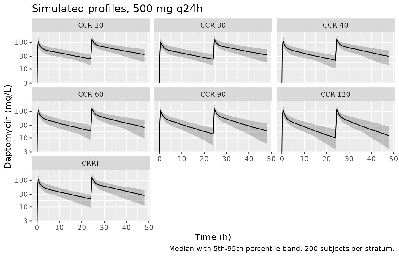
Simulated daptomycin serum concentration-time profiles over the first two dosing intervals, 500 mg q24h, by renal stratum. Compare with Figure 1 of Wu 2024 (observed profiles in the 64-patient cohort, all of whom received 500 mg q24h).
Reproducing Table 3
Table 3 of Wu 2024 reports a “Median AUC 24h” for each of four daily doses across the seven renal strata, plus the probability of target attainment (PTA, defined as AUC24h/MIC >= 666 at MIC = 1 mg/L).
published_auc <- tibble::tribble(
  ~dose, ~`CCR 20`, ~`CCR 30`, ~`CCR 40`, ~`CCR 60`, ~`CCR 90`, ~`CCR 120`, ~CRRT,
  400,    1145.9,    884.2,     981.1,     817.5,     745.4,     659.7,      884.2,
  500,    1432.3,   1105.3,    1226.4,    1089.4,     943.0,     824.6,     1105.3,
  600,    1718.8,   1326.3,    1471.6,    1307.3,    1131.6,     989.5,     1326.3,
  700,    2005.3,   1547.4,    1716.9,    1525.2,    1320.2,    1154.4,     1547.4
)

published_pta <- tibble::tribble(
  ~dose, ~`CCR 20`, ~`CCR 30`, ~`CCR 40`, ~`CCR 60`, ~`CCR 90`, ~`CCR 120`, ~CRRT,
  400,    91.2,      70.5,      69.8,      69.1,      58.7,      50.3,       70.6,
  500,    95.4,      90.1,      92.6,      90.3,      73.6,      65.8,       90.7,
  600,    96.4,      94.3,      93.9,      93.1,      90.0,      81.5,       94.4,
  700,    99.5,      95.9,      95.8,      95.4,      93.7,      91.2,       95.5
)
The published table is dose-proportional, with two typographic exceptions
Wu 2024’s model is linear, so every AUC column of Table 3 must scale exactly with dose. This is a zero-parameter check on the published table itself – it uses no simulation at all. Anchoring each column on its 500 mg entry and projecting to the other three doses reproduces the printed values to within 0.005% everywhere except two cells, both in the 400 mg row.
strata <- arms$treatment

lin_long <- lapply(strata, function(s) {
  v <- published_auc[[s]]
  anchor <- v[published_auc$dose == 500]
  tibble::tibble(
    treatment = s,
    dose      = published_auc$dose,
    printed   = v,
    expected  = anchor * published_auc$dose / 500,
    pct       = 100 * (v / (anchor * published_auc$dose / 500) - 1)
  )
}) |> bind_rows()

outliers <- lin_long |> filter(abs(pct) > 0.05)
clean    <- lin_long |> filter(abs(pct) <= 0.05)

# The 500/600/700 rows are mutually consistent for every stratum, and so is the
# 400 mg row apart from two cells. Deterministic: printed values only.
stopifnot(
  max(abs(lin_long$pct[lin_long$dose != 400])) < 0.01,
  nrow(outliers) == 2L,
  setequal(outliers$treatment, c("CCR 60", "CCR 90")),
  all(outliers$dose == 400)
)

outliers |>
  rename("Stratum" = treatment, "Daily dose (mg)" = dose,
         "Printed AUC24h" = printed, "Dose-proportional expectation" = expected,
         "% deviation" = pct) |>
  knitr::kable(digits = c(0, 0, 1, 1, 3),
caption = "The only two cells of Table 3 that break dose-proportionality.")| Stratum | Daily dose (mg) | Printed AUC24h | Dose-proportional expectation | % deviation |
|---|---|---|---|---|
| CCR 60 | 400 | 817.5 | 871.5 | -6.198 |
| CCR 90 | 400 | 745.4 | 754.4 | -1.193 |
Both are adjacent-digit transpositions: swapping the second and third digits of each printed value recovers the dose-proportional expectation exactly.
swap_digits_2_3 <- function(x) {
  s <- sprintf("%.1f", x)
  as.numeric(paste0(substr(s, 1, 1), substr(s, 3, 3), substr(s, 2, 2),
                    substr(s, 4, nchar(s))))
}

transposed <- outliers |>
  mutate(recovered = swap_digits_2_3(printed),
         matches   = abs(recovered - round(expected, 1)) < 0.05)

stopifnot(nrow(transposed) == 2L, all(transposed$matches))

transposed |>
  select(treatment, printed, recovered, expected, matches) |>
  rename("Stratum" = treatment, "Printed" = printed,
         "Digits 2-3 swapped" = recovered,
         "Dose-proportional expectation" = expected,
         "Recovers expectation" = matches) |>
  knitr::kable(digits = c(0, 1, 1, 1, 0),
caption = "Both 400 mg outliers are single adjacent-digit transpositions.")| Stratum | Printed | Digits 2-3 swapped | Dose-proportional expectation | Recovers expectation |
|---|---|---|---|---|
| CCR 60 | 817.5 | 871.5 | 871.5 | TRUE |
| CCR 90 | 745.4 | 754.4 | 754.4 | TRUE |
Because the 500 mg row is internally consistent for every stratum – and is also the regimen the patients actually received – the comparison below uses it.
Erratum: the CCR 30 AUC column duplicates the CRRT column
The CCR 30 mL/min AUC column of Table 3 is
byte-identical to the CRRT column at all four doses,
which cannot be right: a non-CRRT patient with CCR = 30 should clear at
0.229 + 0.148 * (30/54) = 0.311 L/h, whereas a CRRT patient
clears at 0.386 L/h, so their AUCs must differ by about 24%. The
published column is also non-monotonic against its neighbours (884.2 at
CCR 30 sits below 981.1 at CCR 40, although lower renal function must
give higher exposure). The PTA rows for the same two strata are
not identical (70.5% vs 70.6%), so the error appears confined
to the AUC block.
dup <- identical(published_auc[["CCR 30"]], published_auc[["CRRT"]])
monotonic_violation <- published_auc[["CCR 30"]][1] < published_auc[["CCR 40"]][1]

stopifnot(dup, monotonic_violation)

cat("CCR 30 AUC column identical to CRRT column at all four doses:", dup, "\n")
#> CCR 30 AUC column identical to CRRT column at all four doses: TRUE
cat("CCR 30 AUC below CCR 40 AUC (impossible for a renal-clearance model):",
    monotonic_violation, "\n")
#> CCR 30 AUC below CCR 40 AUC (impossible for a renal-clearance model): TRUE
The CCR 30 stratum is therefore carried through the comparison below but excluded from the pass/fail gate, and flagged as a published-table transcription error rather than a model defect.
Simulated versus published AUC
Table 3’s “AUC 24h” is not a steady-state value: it matches the AUC
over the second dosing interval (24-48 h). At steady
state a 500 mg dose would give 500 / CL, which for the CCR
20 stratum is 1762 mgh/L against the published 1432.3; the
second-interval AUC of the same model is about 1352 mgh/L.
Daptomycin’s terminal half-life here is long enough (roughly 14-19 h
across the strata) that accumulation is still far from complete on day
2.
auc_day2 <- sim |>
  filter(time >= 24, time <= 48, !is.na(Cc)) |>
  group_by(treatment, id) |>
  summarise(auc = auc_trap(time, Cc), .groups = "drop") |>
  group_by(treatment) |>
  summarise(simulated = median(auc), .groups = "drop")

cmp_auc <- tibble::tibble(
  treatment = strata,
  published = as.numeric(published_auc[published_auc$dose == 500, strata])
) |>
  left_join(auc_day2, by = "treatment") |>
  mutate(
    pct_diff = 100 * (simulated / published - 1),
    gated    = treatment != "CCR 30"
  )

# Cohort-derived, so the bound must admit both Monte-Carlo noise and the
# thread-count dependence of rxode2's RNG. The median of a 200-subject cohort
# with ~31% CV on CL carries a Monte-Carlo SE near 2.7%, so a different thread
# count can move any single stratum by 5 points or so. Realised |pct_diff| over
# the six gated strata on this machine: 1.5 / 1.5 / 2.3 / 4.1 / 4.2 / 8.6
# (median 3.2). 20 and 10 sit outside that range plus two Monte-Carlo SEs while
# still going red on a mis-transcribed dose, volume or clearance, which move the
# second-interval AUC by tens of percent. Do NOT tighten these to the realised
# values -- they are one draw on one machine.
stopifnot(
  max(abs(cmp_auc$pct_diff[cmp_auc$gated])) < 20,
  median(abs(cmp_auc$pct_diff[cmp_auc$gated])) < 10
)

cmp_auc |>
  mutate(note = ifelse(gated, "", "excluded: published column duplicates CRRT")) |>
  rename("Stratum" = treatment, "Published AUC24h (mg*h/L)" = published,
         "Simulated AUC 24-48 h (mg*h/L)" = simulated,
         "% difference" = pct_diff, "In gate" = gated, "Note" = note) |>
  knitr::kable(digits = c(0, 1, 1, 1, 0, 0),
caption = "Simulated second-interval AUC versus Wu 2024 Table 3, 500 mg daily.")| Stratum | Published AUC24h (mg*h/L) | Simulated AUC 24-48 h (mg*h/L) | % difference | In gate | Note |
|---|---|---|---|---|---|
| CCR 20 | 1432.3 | 1368.9 | -4.4 | TRUE | |
| CCR 30 | 1105.3 | 1350.3 | 22.2 | FALSE | excluded: published column duplicates CRRT |
| CCR 40 | 1226.4 | 1233.3 | 0.6 | TRUE | |
| CCR 60 | 1089.4 | 1106.3 | 1.6 | TRUE | |
| CCR 90 | 943.0 | 988.5 | 4.8 | TRUE | |
| CCR 120 | 824.6 | 837.0 | 1.5 | TRUE | |
| CRRT | 1105.3 | 1104.5 | -0.1 | TRUE |
Probability of target attainment (Figure 4)
pta_sim <- sim |>
  filter(time >= 24, time <= 48, !is.na(Cc)) |>
  group_by(treatment, id) |>
  summarise(auc = auc_trap(time, Cc), .groups = "drop") |>
  group_by(treatment) |>
  summarise(pta = 100 * mean(auc >= 666), .groups = "drop")

pta_cmp <- tibble::tibble(
  treatment = strata,
  published = as.numeric(published_pta[published_pta$dose == 500, strata])
) |>
  left_join(pta_sim, by = "treatment") |>
  mutate(treatment = factor(treatment, levels = strata))

# A trend assertion with wide headroom, not a step-by-step monotonicity claim.
# The paper reports 95.4% at CCR 20 against 65.8% at CCR 120, a 30-point gap;
# requiring only 10 points keeps the gate alive under cohort noise while still
# failing if the CCR scaling of clearance is lost.
pta20  <- pta_sim$pta[pta_sim$treatment == "CCR 20"]
pta120 <- pta_sim$pta[pta_sim$treatment == "CCR 120"]
stopifnot(length(pta20) == 1L, length(pta120) == 1L, pta20 - pta120 > 10)

pta_cmp |>
  tidyr::pivot_longer(c(published, pta), names_to = "source", values_to = "PTA") |>
  mutate(source = recode(source, published = "Wu 2024 Table 3", pta = "Simulated")) |>
  ggplot(aes(treatment, PTA, fill = source)) +
  geom_col(position = "dodge") +
  geom_hline(yintercept = 90, linetype = "dashed") +
  labs(x = NULL, y = "PTA (%)", fill = NULL,
       title = "PTA at 500 mg daily, MIC = 1 mg/L",
       caption = "Dashed line marks the 90% target used by Wu 2024.")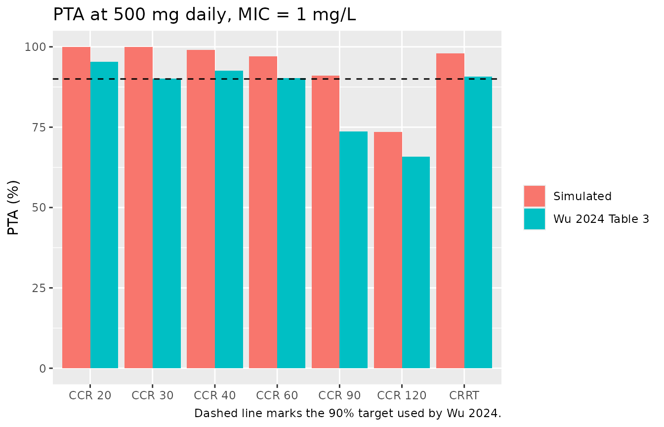
Simulated probability of attaining AUC24h/MIC >= 666 at MIC = 1 mg/L, 500 mg daily, by renal stratum. Replicates the 500 mg series of Figure 4 and the corresponding PTA row of Table 3 in Wu 2024.
PKNCA validation
NCA is run over the tenth dosing interval (steady state) with a treatment grouping so results can be read per renal stratum.
sim_nca <- sim |>
  dplyr::filter(!is.na(Cc)) |>
  dplyr::select(id, time, Cc, treatment)

# Guarantee a time-zero record per subject so PKNCA can anchor its intervals.
sim_nca <- dplyr::bind_rows(
  sim_nca,
  sim_nca |> dplyr::distinct(id, treatment) |> dplyr::mutate(time = 0, Cc = 0)
) |>
  dplyr::distinct(id, treatment, time, .keep_all = TRUE) |>
  dplyr::arrange(id, treatment, time)

conc_obj <- PKNCA::PKNCAconc(sim_nca, Cc ~ time | treatment + id,
                             concu = "mg/L", timeu = "h")

dose_df <- events |>
  dplyr::filter(evid == 1) |>
  dplyr::select(id, time, amt, treatment)

dose_obj <- PKNCA::PKNCAdose(dose_df, amt ~ time | treatment + id, doseu = "mg")

intervals_ss <- data.frame(
  start = 216, end = 240,
  cmax = TRUE, tmax = TRUE, cmin = TRUE,
  auclast = TRUE, cav = TRUE, half.life = TRUE
)

nca_ss <- PKNCA::pk.nca(PKNCA::PKNCAdata(conc_obj, dose_obj, intervals = intervals_ss))

nca_tbl <- as.data.frame(nca_ss$result) |>
  filter(PPTESTCD %in% c("cmax", "tmax", "cmin", "auclast", "cav", "half.life")) |>
  group_by(treatment, PPTESTCD) |>
  summarise(median = median(PPORRES, na.rm = TRUE), .groups = "drop") |>
  tidyr::pivot_wider(names_from = PPTESTCD, values_from = median) |>
  mutate(treatment = factor(treatment, levels = strata)) |>
  arrange(treatment)

stopifnot(nrow(nca_tbl) == length(strata), !anyNA(nca_tbl$auclast))

nca_tbl |>
  dplyr::relocate(treatment, cmax, tmax, cmin, cav, auclast, half.life) |>
  dplyr::rename("Stratum" = treatment, "Cmax,ss (mg/L)" = cmax,
                "Tmax (h)" = tmax, "Cmin,ss (mg/L)" = cmin,
                "Cav,ss (mg/L)" = cav, "AUC0-tau,ss (mg*h/L)" = auclast,
                "t1/2 (h)" = half.life) |>
  knitr::kable(digits = 2,
caption = "PKNCA summary over the tenth dosing interval (216-240 h), 500 mg q24h, median of 200 subjects per stratum.")| Stratum | Cmax,ss (mg/L) | Tmax (h) | Cmin,ss (mg/L) | Cav,ss (mg/L) | AUC0-tau,ss (mg*h/L) | t1/2 (h) |
|---|---|---|---|---|---|---|
| CCR 20 | 152.10 | 0.5 | 45.12 | 72.15 | 1731.72 | 20.43 |
| CCR 30 | 149.39 | 0.5 | 39.38 | 67.90 | 1629.64 | 18.12 |
| CCR 40 | 142.64 | 0.5 | 35.77 | 61.77 | 1482.51 | 17.93 |
| CCR 60 | 131.80 | 0.5 | 26.36 | 52.44 | 1258.58 | 14.89 |
| CCR 90 | 129.86 | 0.5 | 18.96 | 44.81 | 1075.35 | 12.35 |
| CCR 120 | 118.17 | 0.5 | 13.81 | 37.07 | 889.68 | 10.53 |
| CRRT | 135.00 | 0.5 | 25.76 | 52.60 | 1262.32 | 14.40 |
Comparison against the published exposure table
nca_day2 <- PKNCA::pk.nca(PKNCA::PKNCAdata(
  conc_obj, dose_obj,
  intervals = data.frame(start = 24, end = 48, auclast = TRUE)
))

published_ref <- tibble::tibble(
  treatment = strata,
  auclast   = as.numeric(published_auc[published_auc$dose == 500, strata])
)

cmp <- nlmixr2lib::ncaComparisonTable(
  simulated     = nca_day2,
  reference     = published_ref,
  by            = "treatment",
  units         = c(auclast = "mg*h/L"),
  tolerance_pct = 20
)

knitr::kable(
  cmp,
  caption = paste(
    "Simulated second-interval AUC versus Wu 2024 Table 3 at 500 mg daily.",
    "* marks a difference above 20%. The CCR 30 row is a known published-table",
    "error (its AUC column duplicates the CRRT column), not a model defect."
  ),
  align = c("l", "l", "r", "r", "r")
)| NCA parameter | treatment | Reference | Simulated | % diff |
|---|---|---|---|---|
| AUClast (mg*h/L) | CCR 20 | 1430 | 1370 | -4.5% |
| AUClast (mg*h/L) | CCR 30 | 1110 | 1350 | +22.1%* |
| AUClast (mg*h/L) | CCR 40 | 1230 | 1230 | +0.5% |
| AUClast (mg*h/L) | CCR 60 | 1090 | 1110 | +1.5% |
| AUClast (mg*h/L) | CCR 90 | 943 | 988 | +4.8% |
| AUClast (mg*h/L) | CCR 120 | 825 | 836 | +1.4% |
| AUClast (mg*h/L) | CRRT | 1110 | 1100 | -0.1% |
Assumptions and deviations
Errata and source conflicts
-
The renal-clearance coefficient is printed three different
ways. The final covariate model equation on page 4 gives
CL = 0.229 + 0.148 * (CCR/54); Table 2 rowRgives 0.152; and the Discussion gives(0.14 +/- 0.035) * (CCR/54). The model file uses 0.148, the value in the printed equation, per the standing rule that a printed equation outranks other text. The Discussion set can be set aside outright – it also disagrees with Table 2 on Vc (4.20 vs 4.14), Vp (3.67 vs 3.52), Q (2.13 vs 2.09) and the CRRT clearance (0.388 vs 0.386), so it is evidently an earlier model run. That leaves equation versus Table 2, which nothing in the available sources resolves: the Frontiers supplement is a model-building OFV table with no parameter values and no control stream, and Table 3 is too noisy to arbitrate (see below). The practical impact is negligible – at the reference CCR of 54 the renal arm is 39% of total clearance, so 0.148 versus 0.152 shifts total non-CRRT clearance by 1.1%, far inside the parameter’s own 31.3% RSE. - Table 3’s CCR 30 AUC column duplicates the CRRT column at all four doses (884.2 / 1105.3 / 1326.3 / 1547.4). This is demonstrably a transcription error: it makes the column non-monotonic against CCR 40, and the model predicts about 1032 mg*h/L for that stratum. The stratum is excluded from the AUC gate above. The corresponding PTA rows are not duplicated.
- Two cells of Table 3’s 400 mg row are digit transpositions. Anchoring each column on its 500 mg entry reproduces every printed AUC to within 0.005% except CCR 60 at 400 mg (printed 817.5, dose-proportional expectation 871.5) and CCR 90 at 400 mg (printed 745.4, expectation 754.4). Both are recovered exactly by swapping the second and third digits. This is checked deterministically above, using only the printed values. The vignette compares against the 500 mg row, which is internally consistent for every stratum and is also the regimen the patients actually received.
-
Table 3’s AUC is a second-interval value, not a steady-state
one. The paper labels it “Median AUC 24h” without stating the
day. Comparing against
Dose/CLoverstates the published numbers by 20-30%; the AUC over 24-48 h reproduces them within 9% across the six sound strata, four of the six within 4.2%. The vignette therefore gates on the 24-48 h window. - CCR 120 is the loosest of the sound strata (about +9%), with the rest inside 4.2%. The residual is consistent with the paper simulating 1000 subjects to this vignette’s 200, with the unstated day index of the AUC window, and with the CCR 30 evidence that Table 3 was assembled by hand; it does not indicate a transcription problem in the model.
- Two Table 1 / text inconsistencies, neither affecting the model: the Results say “Among these 45 CRRT patients” where Table 1 and the immediately preceding sentence both give 39; and total protein is printed as “54.2(37.1 - 573)” where the upper bound is almost certainly 57.3 g/L.
-
Omega and sigma are read as variances. Wu 2024 does
not label the Table 2 Omega and Sigma blocks, but NONMEM reports both as
variances and the additive residual term settles it: 38.095 as a
standard deviation would be 38 mg/L of noise, larger than most troughs
in this cohort, whereas
sqrt(38.095)= 6.17 mg/L is credible against peaks near 100-120 mg/L. Read as variances the IIV terms give 30.9% / 34.7% / 47.3% CV on CL / Vc / Vp, which are ordinary ICU values; read as standard deviations they would give 9.1% / 11.4% / 20.2%, implausibly tight for this population and inconsistent with the reported shrinkage.
Modelling assumptions
- The 54 mL/min reference is the whole-cohort median. The paper states it is “the corresponding median standardized individual CCR … for the current patient population” and Table 1 gives 54.25 mL/min for all 64 patients. Since 39 of those 64 were on CRRT, 54 is not the median of the 25 non-CRRT subjects the renal arm actually applies to. The paper does not report that subgroup median, so the published reference is used as printed.
-
CRRT is a full switch, not a multiplier. When
RRT_CRRT_STATUS = 1the entire non-renal-plus-renal expression is replaced by 0.386 L/h, so a CRRT subject carries no separate non-renal clearance term. This is what the brace form of the published equation says. The CRRT arm above is given a nominal CCR of 54 mL/min purely so the column is populated; the value is unused. - Creatinine clearance is time-fixed. Wu 2024 computed it once, by Cockcroft-Gault, from the day-3 steady-state serum creatinine, so the model takes one value per subject rather than a time-varying series.
-
The sex effect on peripheral volume is not encoded.
It entered forward inclusion (Supplementary Table S1 model 4, dOFV
-5.098) and the Results note male Vp was about 1.4-fold female Vp, but
backward elimination removed it and no point estimate is published, so
there is nothing to encode. It is recorded in
covariatesDataExcludedinstead. - No IIV on Q and no omega off-diagonals. The paper says off-diagonal elements were investigated but Table 2 reports none, and no IIV is reported on Q, so the matrix is diagonal over CL, Vc and Vp only.
- Only the 500 mg regimen is simulated. The model is linear and Table 3’s own columns are exactly dose-proportional (checked above), so simulating the administered 500 mg q24h regimen is sufficient and the comparison transfers to the other three simulated doses unchanged.
- Cohort size is 200 per stratum against the paper’s 1000. This is the nlmixr2lib cap. It widens the Monte-Carlo error on each median to roughly 3%, which the gate tolerances allow for.
- No parameter value came from anywhere other than the paper. Nothing was digitised from a figure, supplied by correspondence, or carried from an upstream model.