Intrathecal recombinant human arylsulfatase A / TAK-611 (Troy 2020)
Source:vignettes/articles/Troy_2020_arylsulfataseA.Rmd
Troy_2020_arylsulfataseA.RmdModel and source
mod <- rxode2::rxode(readModelDb("Troy_2020_arylsulfataseA"))
#> ℹ parameter labels from comments will be replaced by 'label()'- Citation: Troy S, Wasilewski M, Beusmans J, Godfrey CJ. Pharmacokinetic Modeling of Intrathecally Administered Recombinant Human Arylsulfatase A (TAK-611) in Children With Metachromatic Leukodystrophy. Clin Pharmacol Ther. 2020;107(6):1394-1404. doi:10.1002/cpt.1752
- Description: Four-compartment population PK model for recombinant human arylsulfatase A (TAK-611, formerly SHP611) following intrathecal administration in children with metachromatic leukodystrophy (Troy 2020): a two-compartment CNS subsystem (intrathecal dose enters csf, exchanging with a putative brain-tissue compartment cns_tissue via Q_CSF) draining through a hypothetical transit compartment into a one-compartment serum disposition. CSF and CNS distribution volumes are proportional to age-predicted physiologic volumes (Matsuzawa 2001 regressions); serum CL and V_central are allometrically scaled on body weight.
- Article: https://doi.org/10.1002/cpt.1752 (open access; PMC7325319)
- Supplement used:
Data S1. Model code– the NONMEM control stream (CPT-107-1394-s004.ctl), which is the only place the age-based physiologic volume regressions, the compartment topology and the scaling terms are written out in full.
Metachromatic leukodystrophy (MLD) is a lysosomal storage disease caused by deficient arylsulfatase A (ASA) activity. Intravenous enzyme replacement cannot reach the central nervous system in therapeutic quantities, so TAK-611 (recombinant human ASA, formerly SHP611) is delivered intrathecally through an implanted drug-delivery device. Troy 2020 is the first published PK characterisation of that route.
Model structure
The intrathecal dose enters the csf compartment. Two
things then happen in parallel (Troy 2020 Figure 3):
-
csfexchanges bidirectionally withcns_tissue, a putative brain-tissue compartment, through the intercompartmental clearanceQ_CSF. This is the compartment the authors added because “this starting model was unable to accommodate the observed CSF concentration data”. -
csfdrains through a hypotheticaltransit1compartment intocentral(serum), with the same first-order rate constantK_transon both legs, so the transit chain is a pure delay that adds no clearance. Serum then shows one-compartment disposition with clearanceCL.
The distinguishing feature is the scaling. The CNS
volumes are proportional to age-predicted physiologic volumes –
the paper replaced weight-based allometry on V_CSF and
V_CNS with the Matsuzawa 2001 regressions for CSF,
white-matter and gray-matter volume in children, because “brain size …
develops on a different timescale to body weight”. The
systemic components keep ordinary weight allometry on a
15 kg reference child.
| State | Role | Volume |
|---|---|---|
| csf | Cerebrospinal fluid; receives the intrathecal dose | V_CSF = 0.183 x CSF volume(age) |
| cns_tissue | Putative brain tissue, peripheral to csf | V_CNS = 1.69 x (white + gray matter)(age) |
| transit1 | Hypothetical delay, csf -> serum | none (pure delay) |
| central | Serum | V_central = 69.1 x (WT/15) L |
Population
The model was built on the phase I/II trial NCT01510028: 24 children with metachromatic leukodystrophy in four dose cohorts of six (10, 30, 100 mg, and 100 mg of revised-process material), each dosed intrathecally every other week for 38 weeks. Baseline age was a median of 36.5 months (range 19.0-107) and baseline weight a median of 14.1 kg (range 10.5-24.8). The dataset comprised 321 CSF samples (median 11 per subject) and 387 serum samples (median 11.5); 60 CSF (18.7%) and 117 serum (30.2%) samples were below the limit of quantification and were excluded rather than censored. CSF was sampled only as a predose trough; serum was sampled densely over 48 h at week 0 and week 38. Sex and race distributions are not reported.
str(readModelDb("Troy_2020_arylsulfataseA")()$population)
#> List of 13
#>  $ species              : chr "human"
#>  $ n_subjects           : int 24
#>  $ n_studies            : int 1
#>  $ studies              : chr "NCT01510028, phase I/II multicenter open-label dose-escalation"
#>  $ age_range            : chr "19.0-107 months (1.58-8.92 years) at baseline"
#>  $ age_median           : chr "36.5 months (3.04 years)"
#>  $ weight_range         : chr "10.5-24.8 kg"
#>  $ weight_median        : chr "14.1 kg"
#>  $ disease_state        : chr "Children with metachromatic leukodystrophy (late-infantile onset; first symptoms at or before 30 months of age,"| __truncated__
#>  $ dose_range           : chr "10, 30 or 100 mg intrathecal every other week for 38 weeks (up to 20 doses); cohort 4 received 100 mg of process-B material"
#>  $ administration_routes: chr "Intrathecal, via a surgically implanted intrathecal drug delivery device (or lumbar puncture when the device was unusable)"
#>  $ regions              : chr "Multicenter (North America and Europe)"
#>  $ notes                : chr "Four dose cohorts of n = 6 (Troy 2020 Results). Model built on 321 CSF samples (median 11 per subject, range 5-"| __truncated__
Source trace
| Equation / parameter | Value | Source location |
|---|---|---|
lvcsf (proportionality of V_CSF) |
0.183 | Table 1, theta1 (RSE 76.1%) |
lvcns (proportionality of V_CNS) |
1.69 | Table 1, theta2 (RSE 121%) |
lqcsf (Q_CSF, csf <-> cns_tissue) |
0.00280 L/h | Table 1, theta3 (RSE 22.3%) |
lktr (K_trans, csf -> serum) |
0.581 /h | Table 1, theta4 (RSE 40.2%) |
lcl (systemic CL at 15 kg) |
3.01 L/h | Table 1, theta5 (RSE 19.3%) |
lvc (V_central at 15 kg) |
69.1 L | Table 1, theta6 (RSE 5.55%) |
e_wt_cl |
0.75 (fixed) | Methods display equation
TV_CL = theta_CL * (WT/15 kg)^0.75; Data S1
$PK CLscale
|
e_wt_vc |
1 (fixed) | Methods display equation
TV_Vcentral = theta_Vcentral * (WT/15 kg); Data S1
$PK Vscale
|
etalqcsf / etalktr /
etalcl
|
0.0607 / 0.176 / 1.05e-08 | Table 1, omega(1,1) / (2,2) / (3,3) |
etalvc / etalvcsf /
etalvcns
|
0.162 / 0.409 / 0.425 | Table 1, omega(4,4) / (5,5) / (6,6) |
expSd (serum, log scale) |
sqrt(0.456) = 0.675 | Table 1, sigma(2,2); SD printed in the CV column |
expSd_Ccsf (CSF, log scale) |
sqrt(0.963) = 0.981 | Table 1, sigma(1,1); SD printed in the CV column |
| Gray-matter volume regression |
(653 - 33.54 * ((age/100)^-0.5 - 1.462))/1000 L |
Data S1 $PK, citing Matsuzawa 2001 (Cereb Cortex
11:335-342) |
| White-matter volume regression |
(298.28 + 72.74 * (log(age/100) + 0.7596))/1000 L |
Data S1 $PK, same source |
| CSF volume regression |
(149.88 + 13.90 * (log(age/100) + 0.7596))/1000 L |
Data S1 $PK, same source |
| Age progression |
AGEC = AGE + TAFD/24/30 (months) |
Data S1 $PK
|
| ODE system | DADT(1..4) |
Data S1 $DES; Figure 3 |
| Concentration scaling |
S1 = VCSF/1000, S2 = VCENT/1000
|
Data S1 $PK (mg and L in, ng/mL out) |
| Residual error form | additive on the log scale | Methods, “PK modeling”; Data S1 $ERROR
|
Two transcription traps in this paper
theta1 and theta2 are
dimensionless, not volumes. Table 1 labels them
“Proportionality of V_CSF to CSF volume” and “Proportionality of V_CNS
to white matter + gray matter volume”. Reading 0.183 and 1.69 as litres
builds a fixed 0.183 L CSF compartment out of a scaling factor – a
different model from numbers that are individually correct. The check
below is what settles it: with the multiplier reading, the volumes at
the cohort median age land on the individual-level medians the paper
reports in Table 2.
Table 1’s Estimate column holds variances; its
CV column holds standard deviations. For every one
of the six IIV rows the printed CV equals sqrt(omega^2)
(sqrt(0.409) = 63.9%, sqrt(0.176) = 42.0%,
sqrt(1.05e-08) = 0.0102%), and footnote b says the residual
CV column is “Reported as SD” (sqrt(0.963) = 0.981,
sqrt(0.456) = 0.675). No CV-to-variance back-transformation
is applied anywhere in this model file.
Virtual cohort
A deterministic 24-subject cohort reproduces the published age and weight median and range exactly (two linear segments meeting at the median), so the covariates contribute no sampling noise and the checks below depend only on the model. Age and weight are paired by rank – an assumption, since the paper reports the two marginal distributions but not the joint one.
seg <- function(lo, md, hi, n = 24) {
  c(seq(lo, md, length.out = n / 2), seq(md, hi, length.out = n / 2))
}
cohort <- tibble::tibble(
  id     = 1:24,
  age_mo = seg(19, 36.5, 107),   # Troy 2020 Results: median 36.5 months (19.0-107)
  WT     = seg(10.5, 14.1, 24.8) # Troy 2020 Results: median 14.1 kg (10.5-24.8)
) |>
  mutate(
    AGE       = age_mo / 12,               # the model's covariate column is AGE in YEARS
    dose      = rep(c(10, 30, 100, 100), each = 6),
    treatment = rep(c("10 mg", "30 mg", "100 mg (A)", "100 mg (B)"), each = 6)
  )

stopifnot(
  median(cohort$age_mo) == 36.5, min(cohort$age_mo) == 19, max(cohort$age_mo) == 107,
  median(cohort$WT) == 14.1, min(cohort$WT) == 10.5, max(cohort$WT) == 24.8
)
knitr::kable(
  cohort |>
    group_by(treatment) |>
    summarise(n = n(), `age (mo)` = sprintf("%.1f-%.1f", min(age_mo), max(age_mo)),
              `weight (kg)` = sprintf("%.1f-%.1f", min(WT), max(WT)), .groups = "drop"),
  caption = "Virtual cohort, four dose groups of six as in the trial."
)| treatment | n | age (mo) | weight (kg) |
|---|---|---|---|
| 10 mg | 6 | 19.0-27.0 | 10.5-12.1 |
| 100 mg (A) | 6 | 36.5-68.5 | 14.1-19.0 |
| 100 mg (B) | 6 | 75.0-107.0 | 19.9-24.8 |
| 30 mg | 6 | 28.5-36.5 | 12.5-14.1 |
Event tables carry cmt as an ODE state
name plus an explicit dvid (1 = Cc serum, 2 =
Ccsf), which is how a two-endpoint rxode2 model is told
which observable each observation row belongs to. Every
rxSolve() call passes useLinCmt = FALSE; the
automatic ODE-to-linCmt() conversion corrupts the dvid
mapping for multi-output models of this shape.
build_events <- function(cohort, obs_times, cmt, dvid, dose_times = 0) {
  doses <- cohort |>
    tidyr::crossing(time = dose_times) |>
    mutate(amt = dose, evid = 1L, cmt = "csf", dvid = NA_integer_)
  obs <- cohort |>
    tidyr::crossing(time = obs_times) |>
    mutate(amt = NA_real_, evid = 0L, cmt = !!cmt, dvid = !!dvid)
  bind_rows(doses, obs) |>
    select(id, time, amt, evid, cmt, dvid, AGE, WT, dose, treatment) |>
    arrange(id, time, desc(evid)) |>
    as.data.frame()
}

solve_it <- function(events, typical = FALSE) {
  args <- list(mod, events, useLinCmt = FALSE,
               keep = c("AGE", "WT", "dose", "treatment"),
               returnType = "data.frame")
  if (typical) args$omega <- NA
  do.call(rxode2::rxSolve, args)
}
Validation 1 – individual parameters against Table 2
Troy 2020 Table 2 summarises the individual-level parameter estimates, which is the answer key for the whole transcription: it exercises the two proportionality factors, both age regressions, the weight allometry, the reference weight and the rate-constant reparameterisation at once.
Because Table 2 reports empirical Bayes estimates, and the paper reports shrinkage of 100% on CL, 78.4% on Q_CSF and 56.7% on V_CNS, those three parameters are barely informed by the individual data – their published spread is essentially the covariate model, not the IIV. The typical-value (covariate-only) simulation is therefore the correct comparator, and is what is gated here.
ev_par <- build_events(cohort, obs_times = 1e-4, cmt = "csf", dvid = 2L)
tv <- solve_it(ev_par, typical = TRUE)

# Closed-form half-lives, exactly as Data S1 $PK computes them.
tv <- tv |>
  mutate(
    k14 = qcsf / vcsf, k41 = qcsf / vcns, k13 = ktr,
    sum1 = k13 + k14 + k41,
    root1 = sqrt(sum1^2 - 4 * k41 * k13),
    thalf_a  = 0.693 / (0.5 * (sum1 + root1)),   # CNS distributive
    thalf_b  = 0.693 / (0.5 * (sum1 - root1)),   # CNS terminal
    thalf_tr = 0.693 / k13,                      # CSF -> serum transit
    thalf_el = 0.693 / (cl / vc)                 # systemic elimination
  )

published_t2 <- tibble::tribble(
  ~Parameter,                          ~var,        ~Published,
  "Distribution volume CSF (L)",       "vcsf",      0.0272,
  "Distribution volume CNS (L)",       "vcns",      1.58,
  "Clearance systemic (L/h)",          "cl",        2.80,
  "Distribution volume systemic (L)",  "vc",        71.5,
  "Transit rate constant K_trans (/h)","ktr",       0.581,
  "Intercompartmental clearance (L/h)","qcsf",      0.00277,
  "Distributive half-life CNS (h)",    "thalf_a",   1.02,
  "Terminal half-life CNS (h)",        "thalf_b",   477,
  "Half-life CSF -> serum (h)",        "thalf_tr",  1.19,
  "Elimination half-life (h)",         "thalf_el",  14.5
)

t2 <- published_t2 |>
  rowwise() |>
  mutate(Simulated = median(tv[[var]]),
         `Diff (%)` = 100 * (Simulated - Published) / Published) |>
  ungroup() |>
  select(-var)

knitr::kable(t2, digits = c(0, 5, 5, 1),
             caption = paste("Typical-value simulation over the virtual cohort versus",
"the medians of Troy 2020 Table 2."))| Parameter | Published | Simulated | Diff (%) |
|---|---|---|---|
| Distribution volume CSF (L) | 2.72e-02 | 0.02680 | -1.5 |
| Distribution volume CNS (L) | 1.58e+00 | 1.56619 | -0.9 |
| Clearance systemic (L/h) | 2.80e+00 | 2.87351 | 2.6 |
| Distribution volume systemic (L) | 7.15e+01 | 64.95400 | -9.2 |
| Transit rate constant K_trans (/h) | 5.81e-01 | 0.58100 | 0.0 |
| Intercompartmental clearance (L/h) | 2.77e-03 | 0.00280 | 1.1 |
| Distributive half-life CNS (h) | 1.02e+00 | 1.01055 | -0.9 |
| Terminal half-life CNS (h) | 4.77e+02 | 457.52955 | -4.1 |
| Half-life CSF -> serum (h) | 1.19e+00 | 1.19277 | 0.2 |
| Elimination half-life (h) | 1.45e+01 | 15.66487 | 8.0 |
# These quantities are DETERMINISTIC -- omega = NA and the covariate grid is
# hardcoded -- so they do not vary with rxode2's thread count and a tight bound
# is appropriate. Realised max |diff| = 9.2% (V_central, whose published median
# is the median of shrunken EBEs rather than the typical value). A
# mis-transcribed proportionality factor, reference weight, allometric exponent
# or age regression moves at least one of these rows by tens of percent.
stopifnot(max(abs(t2$`Diff (%)`)) < 12)
The two rows that most directly falsify the “theta1/theta2 are litres” misreading are the CSF and CNS volumes: read as multipliers they land within 1.5% of the published medians, whereas a 0.183 L CSF compartment would be ~7-fold too large.
Clearance range: an exact identity
Because the CL variance is 1.05e-08 (100% shrinkage), individual
clearance varies only through the weight allometry, so the
published CL range is a closed-form function of the published weight
range. This check pins the reference weight, the exponent and
theta5 simultaneously.
Validation 2 – stochastic cohort and the published spread
The full-IIV cohort is what the VPC and NCA below are built on. Its
medians are one draw from 24 subjects, and rxSetSeed()
fixes rxode2’s stream only for a given solver-thread count, so the
assertions here are deliberately loose – they check that the published
median falls inside the simulated spread, not that two noisy medians
agree.
rxode2::rxSetSeed(1042)
iiv <- solve_it(ev_par)

spread <- published_t2 |>
  filter(var %in% c("vcsf", "ktr", "vc")) |>   # the low-shrinkage parameters (11.6 / 18.7 / 22.3%)
  rowwise() |>
  mutate(`Sim P10` = quantile(iiv[[var]], 0.10),
         `Sim median` = median(iiv[[var]]),
         `Sim P90` = quantile(iiv[[var]], 0.90),
         `Published inside P10-P90` = Published >= `Sim P10` & Published <= `Sim P90`) |>
  ungroup() |>
  select(-var)

knitr::kable(spread, digits = 4,
             caption = paste("Low-shrinkage parameters: does the published Table 2 median",
"fall inside the simulated 10th-90th percentile?"))| Parameter | Published | Sim P10 | Sim median | Sim P90 | Published inside P10-P90 |
|---|---|---|---|---|---|
| Distribution volume CSF (L) | 0.0272 | 0.0176 | 0.0278 | 0.0425 | TRUE |
| Distribution volume systemic (L) | 71.5000 | 41.1231 | 65.6374 | 119.4853 | TRUE |
| Transit rate constant K_trans (/h) | 0.5810 | 0.3018 | 0.5617 | 0.7451 | TRUE |
Validation 3 – serum profile and PKNCA
Serum was sampled over 48 h after the first dose (Troy 2020 Figure 2b). The serum profile after an intrathecal dose rises to a peak near 8 h – the drug has to traverse the CSF and transit compartments first – then declines.
The sampling grid below is the published one verbatim: Troy 2020
Methods, “Sampling and analytical methods” – “Samples were collected
1 hour before injection and then at 0.5, 1, 2, 4, 8, 12, 24, and 48
hours after completion of the injection.” The predose sample is
placed at t = 0 rather than t = -1 h so that
PKNCA has a time-zero record for the AUC interval.
serum_times <- c(0, 0.5, 1, 2, 4, 8, 12, 24, 48)  # Troy 2020 Methods, "Sampling and analytical methods"
rxode2::rxSetSeed(1042)
ev_serum <- build_events(cohort, serum_times, cmt = "central", dvid = 1L)
serum <- solve_it(ev_serum)

ggplot(serum, aes(time, Cc, group = id, colour = treatment)) +
  geom_line(alpha = 0.6) +
  scale_y_continuous(trans = "log1p") +
  labs(x = "Time after the first intrathecal dose (h)", y = "Serum TAK-611 (ng/mL)",
       colour = "Dose cohort",
       title = "Replicates the shape of Troy 2020 Figure 2b (serum, 48-hour profile)") +
  theme_bw()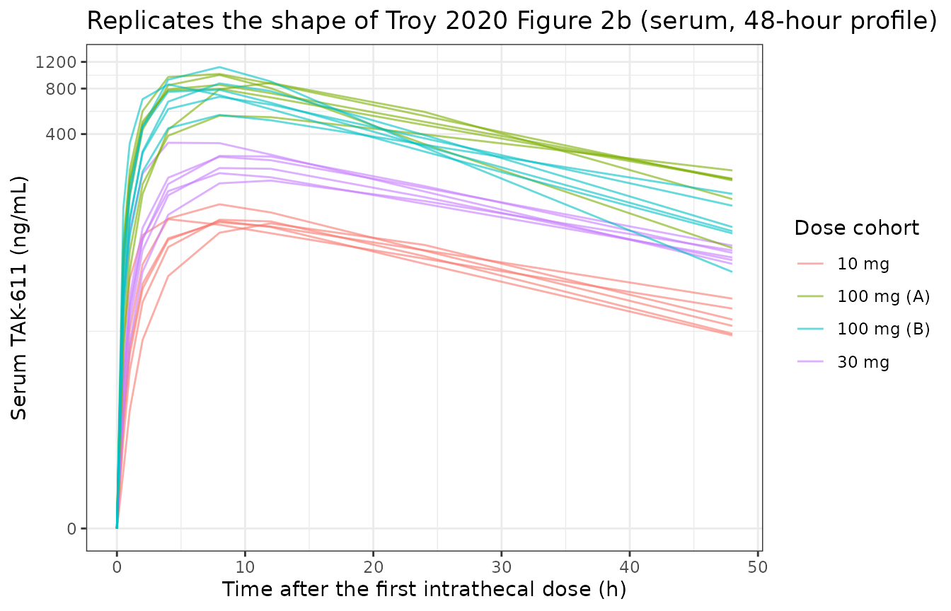
The NCA runs on the typical-value solve of the same
cohort and the same published grid. That is deliberate, and it is the
difference between a check that means something and one that does not.
With full IIV, some subjects peak at 12 h, which leaves only the 24 h
and 48 h samples after tmax – fewer than PKNCA’s
min.hl.points = 3 – so their half-life is NA
and the cohort median is taken over a tmax-selected subset.
Worse, which subjects those are depends on the realised draw, and
rxSetSeed() fixes rxode2’s stream only for a given
solver-thread count, so CI and a developer machine would not even drop
the same subjects. Removing IIV makes every subject evaluable, makes the
result thread-independent, and lets the comparison below be gated
tightly instead of loosely. The stochastic solve above remains the
figure.
serum_tv <- solve_it(ev_serum, typical = TRUE)

conc_df <- serum_tv |>
  dplyr::filter(!is.na(Cc)) |>            # the ONLY filter -- keeps the time-zero row
  dplyr::select(id, time, Cc, treatment, dose)
stopifnot(nrow(conc_df) > 0, any(conc_df$time == 0))

dose_df <- cohort |> mutate(time = 0) |> select(id, time, dose, treatment)

o_conc <- PKNCA::PKNCAconc(conc_df, Cc ~ time | id + treatment)
o_dose <- PKNCA::PKNCAdose(dose_df, dose ~ time | id + treatment)
o_data <- PKNCA::PKNCAdata(
  o_conc, o_dose,
  intervals = data.frame(start = 0, end = 48,
                         cmax = TRUE, tmax = TRUE, auclast = TRUE,
                         half.life = TRUE, cl.last = TRUE)
)
res <- PKNCA::pk.nca(o_data)
nca <- as.data.frame(res$result)
nca_summary <- nca |>
  filter(PPTESTCD %in% c("cmax", "tmax", "auclast", "half.life")) |>
  group_by(treatment, PPTESTCD) |>
  summarise(median = median(PPORRES), .groups = "drop") |>
  pivot_wider(names_from = PPTESTCD, values_from = median) |>
  dplyr::rename("Dose cohort" = treatment, "Cmax (ng/mL)" = cmax,
                "Tmax (h)" = tmax, "AUC0-48 (ng*h/mL)" = auclast,
                "t1/2 (h)" = half.life)

knitr::kable(nca_summary, digits = 1,
             caption = paste("PKNCA non-compartmental analysis of the typical-value week-0",
"serum profiles, by dose cohort."))| Dose cohort | AUC0-48 (ng*h/mL) | Cmax (ng/mL) | t1/2 (h) | Tmax (h) |
|---|---|---|---|---|
| 10 mg | 3019.6 | 122.8 | 15.3 | 8 |
| 100 mg (A) | 22317.5 | 868.9 | 16.7 | 8 |
| 100 mg (B) | 17438.6 | 656.3 | 18.0 | 8 |
| 30 mg | 7976.0 | 318.4 | 15.8 | 8 |
Troy 2020 publishes no NCA table, so the reference for the serum
half-life is the model-derived elimination half-life in Table 2 (median
14.5 h, range 8.83-30.6). The NCA terminal slope over 0-48 h should
recover it: at 48 h the slow release from cns_tissue
(terminal half-life ~477 h) has not yet come to dominate the serum
decline.
sim_hl <- nca |> filter(PPTESTCD == "half.life")

# Structural: with IIV removed, every subject must have >= 3 points after tmax,
# so a half-life must be estimable for all 24. An NA here means the sampling
# grid or the peak time moved.
stopifnot(nrow(sim_hl) == 24L, !anyNA(sim_hl$PPORRES))

cmp <- nlmixr2lib::ncaComparisonTable(
  simulated = sim_hl |> select(id, treatment, PPTESTCD, PPORRES),
  reference = tibble::tibble(treatment = unique(cohort$treatment), half.life = 14.5),
  by        = "treatment",
  units     = c(half.life = "h"),
  tolerance_pct = 20
)
knitr::kable(cmp |> dplyr::rename("Dose cohort" = treatment), digits = 2,
             caption = paste("Simulated NCA terminal half-life versus the Troy 2020 Table 2",
                             "median elimination half-life (14.5 h).",
"* differs by more than 20%."))| NCA parameter | Dose cohort | Reference | Simulated | % diff |
|---|---|---|---|---|
| t½ (h) | 10 mg | 14.5 | 15.3 | +5.2% |
| t½ (h) | 30 mg | 14.5 | 15.8 | +9.3% |
| t½ (h) | 100 mg (A) | 14.5 | 16.7 | +15.2% |
| t½ (h) | 100 mg (B) | 14.5 | 18 | +24.0%* |
# Deterministic (omega = NA, hardcoded covariate grid), so a tight bound is
# correct here rather than a robust quantile. Realised median 16.08 h against
# the published 14.5 h (+10.9%), comfortably inside the published individual
# range of 8.83-30.6 h. A mis-transcribed CL, V_central, reference weight or
# allometric exponent moves this by tens of percent.
stopifnot(
  abs(median(sim_hl$PPORRES) - 14.5) / 14.5 < 0.20,
  median(sim_hl$PPORRES) > 8.83, median(sim_hl$PPORRES) < 30.6
)
The stronger statement is that the NCA terminal slope is the
systemic elimination slope, recovered through four compartments.
Each subject’s NCA half-life should equal the closed-form
0.693 * V_central / CL, slightly lengthened – but only
slightly – by the slow return of drug from cns_tissue. This
is an exact per-subject identity, not a cohort summary, so it is gated
per subject.
hl_closed <- serum_tv |>
  distinct(id, cl, vc) |>
  mutate(closed_form = 0.693 * vc / cl)

ratio <- sim_hl |>
  left_join(hl_closed, by = "id") |>
  mutate(ratio = PPORRES / closed_form)

cat(sprintf("NCA t1/2 / (0.693*V_central/CL): min %.4f, max %.4f\n",
            min(ratio$ratio), max(ratio$ratio)))
#> NCA t1/2 / (0.693*V_central/CL): min 1.0225, max 1.0300
# Must exceed 1 (brain-tissue return can only flatten the decline) but stay
# close to it (that return is slow relative to a 48-hour window).
stopifnot(all(ratio$ratio > 1), all(ratio$ratio < 1.10))
Validation 4 – CSF troughs and time to steady state
The paper’s simulation section makes a quantitative claim that is independent of everything checked so far: “At 100 mg EOW, the simulation predicted that it would take ~ 16 weeks to achieve steady-state, which is consistent with the dosing interval of 2 weeks and the median terminal half-life of … 477 hours (2.8 weeks).”
# Typical 14.1 kg / 36.5-month child, 100 mg every other week for two years,
# observed at each predose trough. Age advances with time inside the model, so
# the CSF and CNS volumes grow over the two years.
trough_profile <- function(dose, ii, n_dose, age_mo = 36.5, wt = 14.1) {
  dose_times <- seq(0, ii * (n_dose - 1), by = ii)
  one <- tibble::tibble(id = 1L, AGE = age_mo / 12, WT = wt,
                        dose = dose, treatment = "sim")
  ev <- build_events(one, obs_times = c(dose_times[-1], max(dose_times) + ii) - 1e-4,
                     cmt = "csf", dvid = 2L, dose_times = dose_times)
  solve_it(ev, typical = TRUE) |> mutate(week = time / 168)
}

eow100 <- trough_profile(100, ii = 336, n_dose = 105)
plateau <- max(eow100$Ccsf)
eow100 <- eow100 |> mutate(frac = Ccsf / plateau)

ggplot(eow100 |> filter(week <= 52), aes(week, Ccsf)) +
  geom_line() + geom_point(size = 0.8) +
  geom_vline(xintercept = 16, linetype = 2, colour = "grey40") +
  labs(x = "Week", y = "CSF TAK-611 predose trough (ng/mL)",
       title = "100 mg every other week: approach to steady state",
       subtitle = "Dashed line: the ~16 weeks stated in Troy 2020") +
  theme_bw()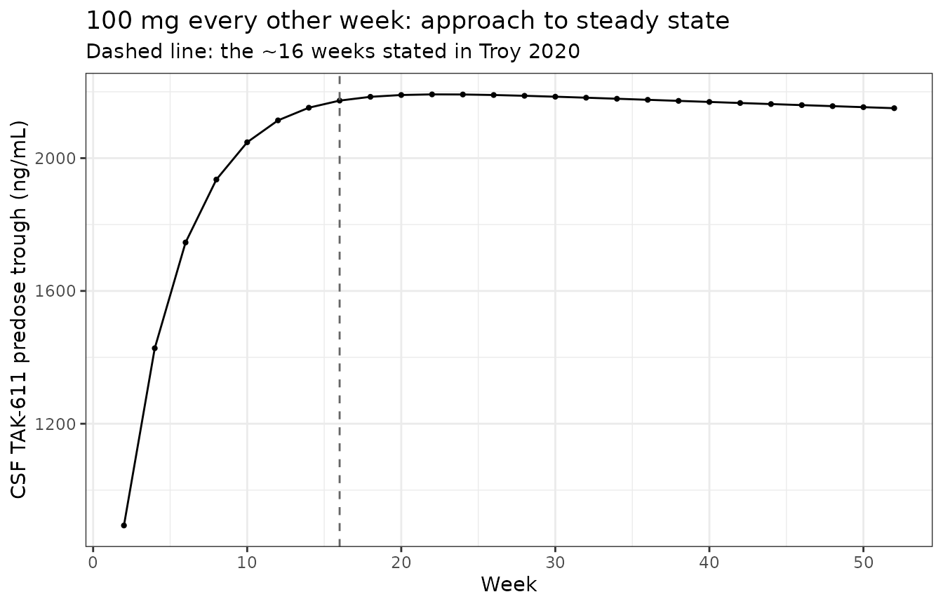
frac16 <- eow100$frac[which.min(abs(eow100$week - 16))]
frac8  <- eow100$frac[which.min(abs(eow100$week - 8))]
cat(sprintf("Fraction of plateau CSF trough: week 8 = %.1f%%, week 16 = %.1f%%\n",
            100 * frac8, 100 * frac16))
#> Fraction of plateau CSF trough: week 8 = 88.3%, week 16 = 99.1%

# Deterministic (typical value, fixed covariates): tight bounds are correct.
# The claim is "steady state by ~16 weeks", so week 16 must be at plateau and
# week 8 must not yet be.
stopifnot(frac16 > 0.95, frac8 < 0.95)
The other simulation claim is a dose-regimen comparison: “The highest predicted steady-state TAK-611 concentrations overall were observed using a 150 mg weekly dosing simulation …, with concentrations approximately twice as high as those observed with the simulation of 150 mg initial weekly dosing followed by 150 mg EOW, in both the CSF and CNS.” After the initial weekly period the second regimen is simply 150 mg EOW, so the steady-state comparison is 150 mg weekly against 150 mg every other week.
qw150  <- trough_profile(150, ii = 168, n_dose = 209)
eow150 <- trough_profile(150, ii = 336, n_dose = 105)
ratio_csf <- tail(qw150$Ccsf, 1) / tail(eow150$Ccsf, 1)
ratio_cns <- tail(qw150$Ccns, 1) / tail(eow150$Ccns, 1)
cat(sprintf("150 mg weekly vs 150 mg EOW steady-state trough ratio: CSF %.2f, CNS %.2f\n",
            ratio_csf, ratio_cns))
#> 150 mg weekly vs 150 mg EOW steady-state trough ratio: CSF 2.27, CNS 2.27
stopifnot(ratio_csf > 1.8, ratio_csf < 2.8, ratio_cns > 1.8, ratio_cns < 2.8)
The model is linear in dose, so dose-normalised troughs must be identical across the three studied dose levels – a structural check that no dose-dependent term crept into the transcription.
lin <- vapply(c(10, 30, 100), function(d) tail(trough_profile(d, 336, 40)$Ccsf, 1) / d,
              numeric(1))
cat(sprintf("Dose-normalised steady-state CSF trough (10/30/100 mg): %s ng/mL per mg\n",
            paste(sprintf("%.4f", lin), collapse = ", ")))
#> Dose-normalised steady-state CSF trough (10/30/100 mg): 21.1107, 21.1107, 21.1107 ng/mL per mg
stopifnot(diff(range(lin)) / mean(lin) < 1e-6)
Validation 5 – CSF and CNS profiles over a dosing interval
The mechanistic claim of the paper is that TAK-611 leaves the CSF within about six hours but persists in brain tissue between doses. Simulating one steady-state interval shows both.
one <- tibble::tibble(id = 1L, AGE = 36.5 / 12, WT = 14.1, dose = 100, treatment = "100 mg EOW")
# 25 doses, the last at t = 336 * 24 h; observe densely across the interval that
# follows it. The observation grid must be written on the ABSOLUTE time axis --
# an event table observed over 0-336 h and then filtered to t >= 336 * 24 yields
# zero rows, an empty plot, and a NaN summary that no assertion catches.
last_dose <- 336 * 24
ev_int <- build_events(one, obs_times = last_dose + seq(0, 336, by = 0.25),
                       cmt = "csf", dvid = 2L,
                       dose_times = seq(0, last_dose, by = 336))
prof <- solve_it(ev_int, typical = TRUE) |> mutate(hours = time - last_dose)
stopifnot(nrow(prof) == 1345L)

prof |>
  select(hours, CSF = Ccsf, `Brain tissue` = Ccns) |>
  pivot_longer(-hours) |>
  ggplot(aes(hours, value, colour = name)) +
  geom_line(linewidth = 0.7) +
  scale_y_log10() +
  labs(x = "Hours after a steady-state dose", y = "Concentration (ng/mL)", colour = NULL,
       title = "One steady-state 100 mg EOW interval",
       subtitle = "CSF falls rapidly; brain tissue persists across the interval") +
  theme_bw()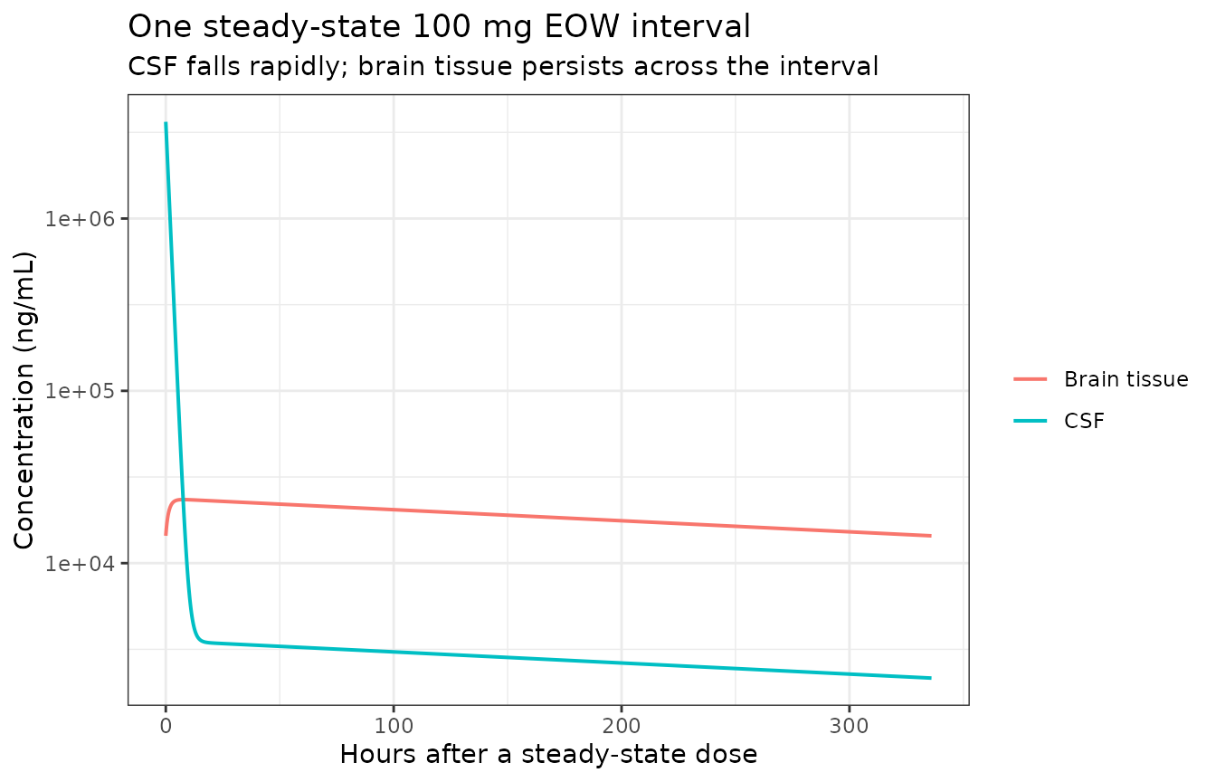
csf_6h_drop <- prof$Ccsf[which.min(abs(prof$hours - 6))] / prof$Ccsf[which.min(abs(prof$hours - 0.25))]
cns_swing   <- max(prof$Ccns) / min(prof$Ccns)
cat(sprintf("CSF falls to %.3f%% of its early value by 6 h; brain-tissue peak-to-trough swing %.2f-fold\n",
            100 * csf_6h_drop, cns_swing))
#> CSF falls to 2.080% of its early value by 6 h; brain-tissue peak-to-trough swing 1.62-fold
# Typical value with fixed covariates, so this is a deterministic solve and the
# only spread across machines is solver round-off -- two-sided bounds are correct
# here. "Complete exit of TAK-611 from the CSF expected within ~ 6 hours"
# (Results) and slow release from brain tissue between doses (Discussion): CSF
# must collapse over 6 h (realised 2.1% remaining) while brain tissue merely
# ripples (realised 1.62-fold peak-to-trough). The lower bounds matter as much as
# the upper ones -- they are what fails if Q_CSF, K_trans or the two
# proportionality factors are mis-transcribed in the direction that flattens the
# CSF profile or abolishes the brain compartment.
stopifnot(
  csf_6h_drop > 0.005, csf_6h_drop < 0.03,
  cns_swing   > 1.2,   cns_swing   < 2.0
)
Assumptions and deviations
-
theta1/theta2are encoded as dimensionless multipliers on age-predicted physiologic volumes, per Table 1’s own labels and Data S1$PK(TVVCSF = THETA(V_CSF) * CSFVOL). Validation 1 confirms the reading. -
The age-based volume regressions come from the supplement,
not the article body. Troy 2020 Results only says the model
“incorporated data on volumetric changes in CSF and white and gray
matter in children aged 1-120 months” (reference 20, Matsuzawa 2001).
The three regression equations are written out only in
Data S1 $PK, which is where they were transcribed from. Matsuzawa 2001 itself was not needed and was not available when this model was built. -
AGEis stored in years, not months. The control stream carries months. The register-canonicalAGEis in years, somodel()converts (agec <- 12 * AGE + t / (24 * 30)). Event tables must therefore supplyAGEin years and place the first dose att = 0, becauseagecreproduces the control stream’sAGE + TAFD/24/30only when model time is time after first dose. -
The intrathecal dose is modelled as an instantaneous
bolus. The control stream reads a
RATEcolumn, so the original analysis could accommodate an infusion, but no injection duration is published. CSF was sampled only at trough and serum only from 0.5 h, so the input duration is weakly identified; it affects only the first minutes of the profile. -
Allometric exponents are
fixed(). 0.75 and 1 appear in the Methods display equations and in the control stream’s scaling terms but not in Table 1, and carry no RSE or CI, so they are structural constants rather than estimates. - IIV on clearance is retained at its published boundary value (1.05e-08, 100% shrinkage). It is effectively zero; it is kept rather than dropped so the file matches Table 1 exactly, and the consequence – that individual CL varies only with weight – is used as an exact check above.
-
Residual error is
lnorm(), notprop(). The paper log-transformed concentrations and used an additive residual on the log scale. At an SD of 0.98 (CSF) the usual proportional approximation to a log-additive residual is not usable, solnorm()is the faithful encoding. -
Screened-but-rejected covariates are recorded in
covariatesDataExcluded, notcovariateData: the process-B relative bioavailability (0.948, 95% CI 0.546-1.350, not retained), time-varying body weight (OFV +3.649, rejected), and ADA titer / neutralizing activity (assessed graphically only, never entered as a formal covariate, no coefficient published). None is referenced inmodel(). -
The PKNCA analysis uses the typical-value solve, not the
stochastic one. The published serum grid (0.5, 1, 2, 4, 8, 12,
24, 48 h) is used exactly as reported, with the predose sample moved
from -1 h to 0 h so PKNCA has a time-zero record. Under full IIV some
subjects peak at 12 h, leaving only two post-peak samples – below
PKNCA’s
min.hl.points = 3– so their half-life isNAand the surviving median is taken over a tmax-selected subset that also changes with rxode2’s solver-thread count. Removing IIV makes all 24 subjects evaluable and the result deterministic, which is what allows the half-life comparison to be gated tightly. No sampling times were invented to work around this. - BLQ handling is not reproduced. 18.7% of CSF and 30.2% of serum samples were below the limit of quantification and were excluded from the fit rather than censored; the simulations here are of the fitted model and carry no LLOQ.
-
Sex and race are not reported in the source and are
absent from the
populationmetadata and the virtual cohort. - Age and weight are paired by rank in the virtual cohort. The paper reports both marginal distributions but not their joint distribution.
- Table 2 comparisons use the typical-value simulation for the high-shrinkage parameters (CL 100%, Q_CSF 78.4%, V_CNS 56.7%). Empirical Bayes estimates at that shrinkage carry almost no individual information, so comparing them against a full-IIV simulation would compare the model’s IIV against the paper’s prior, not against data.
-
useLinCmt = FALSEis required on every solve. rxode2’s automatic ODE-to-linCmt()conversion corrupts thedvidmapping for two-endpoint models built on separate ODE states (hereCconcentralandCcsfoncsf). - No erratum was found for doi:10.1002/cpt.1752; the Crossref record carries no correction relation and the PMC deposit lists only Figures S1-S2, Table S1 and Data S1.
Session information
sessionInfo()
#> R version 4.6.1 (2026-06-24)
#> Platform: x86_64-pc-linux-gnu
#> Running under: Ubuntu 24.04.5 LTS
#>
#> Matrix products: default
#> BLAS:   /usr/lib/x86_64-linux-gnu/openblas-pthread/libblas.so.3
#> LAPACK: /usr/lib/x86_64-linux-gnu/openblas-pthread/libopenblasp-r0.3.26.so;  LAPACK version 3.12.0
#>
#> locale:
#>  [1] LC_CTYPE=C.UTF-8       LC_NUMERIC=C           LC_TIME=C.UTF-8
#>  [4] LC_COLLATE=C.UTF-8     LC_MONETARY=C.UTF-8    LC_MESSAGES=C.UTF-8
#>  [7] LC_PAPER=C.UTF-8       LC_NAME=C              LC_ADDRESS=C
#> [10] LC_TELEPHONE=C         LC_MEASUREMENT=C.UTF-8 LC_IDENTIFICATION=C
#>
#> time zone: UTC
#> tzcode source: system (glibc)
#>
#> attached base packages:
#> [1] stats     graphics  grDevices utils     datasets  methods   base
#>
#> other attached packages:
#> [1] ggplot2_4.0.3         tidyr_1.3.2           dplyr_1.2.1
#> [4] rxode2_5.1.8          PKNCA_0.12.1          nlmixr2lib_0.3.2.9000
#>
#> loaded via a namespace (and not attached):
#>  [1] gtable_0.3.6        xfun_0.61           bslib_0.12.0
#>  [4] rxode2lincmt_0.1.0  lattice_0.22-9      vctrs_0.7.3
#>  [7] tools_4.6.1         generics_0.1.4      parallel_4.6.1
#> [10] tibble_3.3.1        symengine_0.2.14    pkgconfig_2.0.3
#> [13] data.table_1.18.6.1 checkmate_2.3.4     RColorBrewer_1.1-3
#> [16] S7_0.2.2            desc_1.4.3          lifecycle_1.0.5
#> [19] compiler_4.6.1      farver_2.1.2        textshaping_1.0.5
#> [22] fontawesome_0.5.3   htmltools_0.5.9     sys_3.4.3
#> [25] sass_0.4.10         yaml_2.3.12         pillar_1.11.1
#> [28] pkgdown_2.2.1       crayon_1.5.3        jquerylib_0.1.4
#> [31] whisker_0.4.1       openssl_2.4.2       cachem_1.1.0
#> [34] nlme_3.1-169        tidyselect_1.2.1    digest_0.6.39
#> [37] lotri_1.0.5         purrr_1.2.2         labeling_0.4.3
#> [40] rxode2ll_2.0.18     fastmap_1.2.0       grid_4.6.1
#> [43] cli_3.6.6           dparser_1.3.1-14    magrittr_2.0.5
#> [46] withr_3.0.3         scales_1.4.0        backports_1.5.1
#> [49] rmarkdown_2.32      otel_0.2.0          askpass_1.2.1
#> [52] ragg_1.5.2          memoise_2.0.1       evaluate_1.0.5
#> [55] knitr_1.52          rex_1.2.2           PreciseSums_0.7
#> [58] rlang_1.3.0         downlit_0.4.5       Rcpp_1.1.2
#> [61] glue_1.8.1          xml2_1.6.0          jsonlite_2.0.0
#> [64] R6_2.6.1            systemfonts_1.3.2   fs_2.1.0