Mirikizumab in pediatric ulcerative colitis (Otani 2025)
Source:vignettes/articles/Otani_2025_mirikizumab.Rmd
Otani_2025_mirikizumab.Rmd
library(nlmixr2lib)
library(PKNCA)
#>
#> Attaching package: 'PKNCA'
#> The following object is masked from 'package:stats':
#>
#>     filter
library(rxode2)
#> rxode2 5.1.8 using 2 threads (see ?getRxThreads)
#>   no cache: create with `rxCreateCache()`
library(dplyr)
#>
#> Attaching package: 'dplyr'
#> The following objects are masked from 'package:stats':
#>
#>     filter, lag
#> The following objects are masked from 'package:base':
#>
#>     intersect, setdiff, setequal, union
library(tidyr)
library(ggplot2)
Model and source
Otani et al. (2025) characterised the population PK of mirikizumab, a humanised IgG4 anti-IL-23p19 monoclonal antibody, in children and adolescents (2 to <18 years, > 10 kg) with moderately to severely active ulcerative colitis in the open-label phase II SHINE-1 study (NCT04004611). The adult LUCENT 1+2 model (Chua 2023) was the starting point: a linear two-compartment model with first-order absorption of subcutaneous (SC) doses. In the pediatric fit the allometric exponents were fixed (0.8 on CL and Q, 1.0 on the volumes), Ka and Q were fixed to the adult estimates, and time-varying albumin was the only covariate retained besides weight.
The paper did not model exposure-response in children: the narrow exposure range allowed only an exposure-quartile summary of the observed efficacy endpoints (Figure 4) and an overlay on the adult AMAC exposure-response model (Figure 5). The PK model is the only model in the paper.
- Citation: Otani Y, Chua L, Komocsar WJ, Larkin A, Johns J, Zhang XC. Mirikizumab pharmacokinetics and exposure-response in pediatric patients with moderate-to-severe ulcerative colitis. CPT Pharmacometrics Syst Pharmacol. 2025;14(3):474-485. doi:10.1002/psp4.13286
- Article: https://doi.org/10.1002/psp4.13286
Population
Baseline characteristics from Otani 2025 Table 1:
| Characteristic | 5 mg/kg IV (<= 40 kg) | 10 mg/kg IV (<= 40 kg) | 300 mg IV (> 40 kg) | Total |
|---|---|---|---|---|
| N | 10 | 5 | 11 | 26 |
| Age, mean (SD), years | 9.6 (4.2) | 11.6 (1.1) | 14.0 (1.3) | 11.8 (3.4) |
| Male, % | 40.0 | 40.0 | 45.5 | 42.3 |
| White / Asian / Other, % | 50 / 40 / 10 | 60 / 40 / 0 | 90 / 10 / 0 | 68 / 28 / 4 |
| Weight, mean (SD), kg | 28.6 (9.0) | 33.0 (2.4) | 54.7 (13.3) | 40.5 (16.0) |
| Weight <= 20 kg, n | 2 | 0 | 0 | 2 |
| BMI, mean (SD), kg/m^2 | 15.8 (2.3) | 17.0 (0.6) | 21.1 (5.0) | 18.3 (4.3) |
Induction was IV every 4 weeks (weeks 0, 4 and 8) by weight group:
300 mg for > 40 kg, 5 or 10 mg/kg for > 20 to <= 40 kg, 5 mg/kg
for <= 20 kg. Maintenance was SC every 4 weeks from week 12 to week
48 by weight at week 12: 200 mg for > 40 kg, 100 mg for > 20 to
<= 40 kg, 50 mg for <= 20 kg. Week-12 non-responders received
three more IV doses before maintenance. The analysis used 232 serum
samples; six troughs below the limit of quantification were excluded
(226 observations in the final fit). The same information is in the
model’s population metadata.
Source trace
The final estimates come from the NONMEM output in Appendix S1 (supplement 2), which gives them to one more digit than Table 2. Rate constants and clearances are published per hour and are multiplied by 24 to give the per-day values used in the model file.
| Quantity | Value | Source |
|---|---|---|
| Two-compartment, first-order SC absorption, IV into central | ADVAN4 TRANS4 | Methods (Dose selection, Population PK analysis); Appendix S1 |
| Ka (1/h) | 0.00706, fixed | Appendix S1 THETA2; Table 2 footnote c |
| CL (L/h) | 0.0209 | Appendix S1 THETA3; Table 2 (0.021) |
| Vc = V2 (L) | 3.48 | Appendix S1 THETA4; Table 2 |
| Q (L/h) | 0.0087, fixed | Appendix S1 THETA5; Table 2 footnote c |
| Vp = V3 (L) | 1.40 | Appendix S1 THETA6; Table 2 |
| F1 | 0.498, estimated on the logit scale | Appendix S1 THETA1 and $PK; Table 2 footnote f |
| Weight on CL and Q | (WT/70.7)^0.8, fixed | Appendix S1 THETA9 and $PK; Table 2 footnote d |
| Weight on Vc and Vp | (WT/70.7)^1.0, fixed | Appendix S1 THETA10 and $PK; Table 2 footnote e |
| Albumin on CL | 1 + (-0.0218)(ALB - 45) | Appendix S1 THETA11 and $PK; Table 2 footnote d |
| IIV on CL (variance) | 0.128 (37.1%) | Appendix S1 OMEGA3; Table 2 |
| IIV on logit F1 (variance) | 0.471 (77.6%) | Appendix S1 OMEGA1; Table 2 |
| Proportional residual error | 0.288 (SIGMA fixed to 1) | Appendix S1 THETA7 and $ERROR |
| Additive residual error | 0, fixed (not carried) | Appendix S1 THETA8 |
Table 2 footnote b converts each variance as 100 sqrt(exp(OMEGA) - 1), including the logit-scale variance of F1. The check below confirms that the model-file variances reproduce the published percentages and the weight-normalised summary values in the Results. The CL variance printed in Appendix S1 (0.128) gives 37.0% rather than the 37.1% in Table 2 (which would correspond to a variance of 0.129). The model uses the NONMEM output value; the 0.1-point difference has no practical effect.
mod <- readModelDb("Otani_2025_mirikizumab")
ui <- rxode2::rxode(mod)
#> ℹ parameter labels from comments will be replaced by 'label()'
th <- ui$theta
om <- ui$omega

iiv_pct <- c(
  CL = 100 * sqrt(exp(om["etalcl", "etalcl"]) - 1),
  F1 = 100 * sqrt(exp(om["etalogitfdepot", "etalogitfdepot"]) - 1)
)
cl_h <- exp(th[["lcl"]]) / 24
vss_per_kg <- (exp(th[["lvc"]]) + exp(th[["lvp"]])) / 70.7
f_pct <- 100 * plogis(th[["logitfdepot"]])

knitr::kable(
  tibble::tribble(
    ~Quantity, ~Model, ~Published,
    "IIV CL (%)", iiv_pct[["CL"]], 37.1,
    "IIV F1 (%)", iiv_pct[["F1"]], 77.6,
    "CL at 70.7 kg (L/h)", cl_h, 0.021,
    "Vss per kg at 70.7 kg (L/kg)", vss_per_kg, 0.069,
    "SC bioavailability (%)", f_pct, 49.8
  ),
  digits = 4,
  caption = "Model values against Table 2 and the Results text."
)| Quantity | Model | Published |
|---|---|---|
| IIV CL (%) | 36.9531 | 37.100 |
| IIV F1 (%) | 77.5626 | 77.600 |
| CL at 70.7 kg (L/h) | 0.0209 | 0.021 |
| Vss per kg at 70.7 kg (L/kg) | 0.0690 | 0.069 |
| SC bioavailability (%) | 49.8000 | 49.800 |
Virtual cohort
Subject-level data are not public. Each SHINE-1 dose group gets 200 virtual patients, with weights drawn from a normal distribution with the Table 1 mean and SD for that group, truncated to the group’s weight band (which raises the mean of the > 40 kg group by a few kilograms). Albumin was not reported for the pediatric cohort and is held at the 45 g/L reference value.
set.seed(20250315)
rxode2::rxSetSeed(20250315)

draw_weight <- function(n, mean, sd, lower, upper) {
  out <- numeric(0)
  while (length(out) < n) {
    x <- rnorm(4 * n, mean, sd)
    out <- c(out, x[x > lower & x <= upper])
  }
  out[seq_len(n)]
}

n_arm <- 200
groups <- tibble::tribble(
  ~group, ~wt_mean, ~wt_sd, ~wt_lower, ~wt_upper,
  "> 40 kg: 300 mg IV", 54.7, 13.3, 40, 90,
  "<= 40 kg: 5 mg/kg IV", 28.6, 9.0, 12, 40,
  "<= 40 kg: 10 mg/kg IV", 33.0, 2.4, 20, 40
)

cohort <- groups |>
  mutate(arm = row_number()) |>
  rowwise() |>
  reframe(
    group = group,
    arm = arm,
    WT = draw_weight(n_arm, wt_mean, wt_sd, wt_lower, wt_upper)
  ) |>
  mutate(
    id = row_number(),
    ALB = 45,
    group = factor(group, levels = groups$group),
    iv_dose = case_when(
      arm == 1 ~ 300,
      arm == 2 ~ 5 * WT,
      arm == 3 ~ 10 * WT
    ),
    sc_dose = case_when(WT > 40 ~ 200, WT > 20 ~ 100, TRUE ~ 50)
  )

cohort |>
  group_by(group) |>
  summarise(
    n = n(),
    mean_wt = mean(WT),
    sd_wt = sd(WT),
    min_wt = min(WT),
    max_wt = max(WT)
  ) |>
  rename(
    "Dose group" = group,
    N = n,
    "Mean weight (kg)" = mean_wt,
    "SD weight (kg)" = sd_wt,
    "Min weight (kg)" = min_wt,
    "Max weight (kg)" = max_wt
  ) |>
knitr::kable(digits = 1, caption = "Virtual SHINE-1 cohort.")| Dose group | N | Mean weight (kg) | SD weight (kg) | Min weight (kg) | Max weight (kg) |
|---|---|---|---|---|---|
| > 40 kg: 300 mg IV | 200 | 58.2 | 10.2 | 40.3 | 81.6 |
| <= 40 kg: 5 mg/kg IV | 200 | 28.3 | 6.4 | 12.9 | 39.9 |
| <= 40 kg: 10 mg/kg IV | 200 | 32.9 | 2.4 | 25.5 | 39.0 |
SHINE-1 regimen over 52 weeks (Figure 2)
Each virtual patient receives three IV induction doses (weeks 0, 4 and 8, 40-minute infusions) followed by SC maintenance every 4 weeks from week 12 to week 48 at the dose for their weight. The figure shows the median and 90% prediction interval of the simulated concentrations, the quantities whose observed counterparts the prediction-corrected VPC in Figure 2 of Otani 2025 compares.
inf_dur <- 40 / 1440

regimen_events <- bind_rows(
  tidyr::expand_grid(cohort, time = c(0, 28, 56)) |>
    mutate(evid = 1L, amt = iv_dose, rate = iv_dose / inf_dur, cmt = "central"),
  tidyr::expand_grid(cohort, time = seq(84, 336, by = 28)) |>
    mutate(evid = 1L, amt = sc_dose, rate = 0, cmt = "depot"),
  tidyr::expand_grid(cohort, time = seq(0, 364, by = 1)) |>
    mutate(evid = 0L, amt = 0, rate = 0, cmt = "central")
) |>
  select(id, time, evid, amt, rate, cmt, WT, ALB, group) |>
  arrange(id, time, desc(evid))

sim_regimen <- rxode2::rxSolve(
  mod,
  events = regimen_events,
  keep = "group",
  returnType = "data.frame"
)
#> ℹ parameter labels from comments will be replaced by 'label()'
sim_regimen |>
  group_by(group, time) |>
  summarise(
    q05 = quantile(Cc, 0.05),
    q50 = median(Cc),
    q95 = quantile(Cc, 0.95),
    .groups = "drop"
  ) |>
  filter(time > 0) |>
  ggplot(aes(time / 7, q50, colour = group, fill = group)) +
  geom_ribbon(aes(ymin = q05, ymax = q95), alpha = 0.2, colour = NA) +
  geom_line() +
  scale_y_log10() +
  scale_x_continuous(breaks = seq(0, 52, by = 4)) +
  labs(
    x = "Time (weeks)",
    y = "Mirikizumab concentration (ug/mL)",
    colour = "Induction group", fill = "Induction group",
    caption = paste(
      "Simulated SHINE-1 regimen (median and 90% PI);",
      "compare with Figure 2 of Otani 2025."
    )
  ) +
  theme_bw() +
  theme(legend.position = "bottom")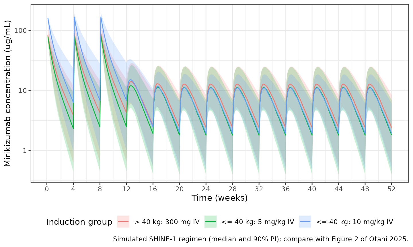
Steady-state exposure by dose group (Figure 3)
Figure 3 of Otani 2025 shows the model-estimated steady-state Cmax, AUC over the 4-week dosing interval and Cavg for each pediatric weight and dose group. Steady state is reached here with explicit dose trains: six IV doses every 4 weeks for induction, and ten SC doses every 4 weeks for maintenance. NCA is taken over the last interval of each. Maintenance groups are defined by weight band, as in the figure: > 40 kg receiving 200 mg and > 20 to <= 40 kg receiving 100 mg. The same patients are re-used, so the maintenance groups pool the induction arms by weight.
iv_ss <- tidyr::expand_grid(cohort, dose_no = 0:5) |>
  mutate(
    time = 28 * dose_no,
    evid = 1L,
    amt = iv_dose,
    rate = iv_dose / inf_dur,
    cmt = "central",
    treatment = paste("Induction:", group)
  )
iv_obs <- tidyr::expand_grid(
  cohort,
  time = c(0, seq(140, 168, by = 0.25), 140 + inf_dur)
) |>
  mutate(
    evid = 0L,
    amt = 0,
    rate = 0,
    cmt = "central",
    treatment = paste("Induction:", group)
  )

sc_cohort <- cohort |>
  filter(WT > 20) |>
  mutate(
    id = id + nrow(cohort),
    treatment = ifelse(
      WT > 40,
      "Maintenance: > 40 kg: 200 mg SC",
      "Maintenance: > 20 to <= 40 kg: 100 mg SC"
    )
  )
sc_ss <- tidyr::expand_grid(sc_cohort, dose_no = 0:9) |>
  mutate(time = 28 * dose_no, evid = 1L, amt = sc_dose, rate = 0, cmt = "depot")
sc_obs <- tidyr::expand_grid(sc_cohort, time = c(0, seq(252, 280, by = 0.25))) |>
  mutate(evid = 0L, amt = 0, rate = 0, cmt = "central")

ss_events <- bind_rows(iv_ss, iv_obs, sc_ss, sc_obs) |>
  select(id, time, evid, amt, rate, cmt, WT, ALB, treatment) |>
  distinct(id, time, evid, .keep_all = TRUE) |>
  arrange(id, time, desc(evid))

sim_ss <- rxode2::rxSolve(
  mod,
  events = ss_events,
  keep = "treatment",
  returnType = "data.frame"
)
sim_nca <- sim_ss |>
  filter(!is.na(Cc)) |>
  select(id, time, Cc, treatment)

dose_nca <- ss_events |>
  filter(evid == 1) |>
  select(id, time, amt, treatment)

intervals <- data.frame(
  treatment = sort(unique(sim_nca$treatment)),
  cmax = TRUE,
  auclast = TRUE,
  cav = TRUE
) |>
  mutate(
    start = ifelse(grepl("^Induction", treatment), 140, 252),
    end = start + 28
  )

conc_obj <- PKNCA::PKNCAconc(sim_nca, Cc ~ time | treatment + id)
dose_obj <- PKNCA::PKNCAdose(dose_nca, amt ~ time | treatment + id)
nca_res <- PKNCA::pk.nca(
  PKNCA::PKNCAdata(conc_obj, dose_obj, intervals = intervals)
)
Comparison against Figure 3
The reference values are the box-plot medians of Figure 3, read from the figure by the maintainers; reading error is a few percent. Figure 3 summarises the individual estimates of the 26 participants (2 to 11 per group), so each reference median is itself uncertain.
fig3_medians <- tibble::tribble(
  ~treatment, ~cmax, ~auclast, ~cav,
  "Induction: > 40 kg: 300 mg IV", 122, 700, 25.5,
  "Induction: <= 40 kg: 5 mg/kg IV", 107, 520, 19,
  "Induction: <= 40 kg: 10 mg/kg IV", 212, 1560, 56,
  "Maintenance: > 40 kg: 200 mg SC", 15, 230, 8.2,
  "Maintenance: > 20 to <= 40 kg: 100 mg SC", 12.5, 225, 8.0
)

cmp <- nlmixr2lib::ncaComparisonTable(
  simulated = nca_res,
  reference = fig3_medians,
  by = "treatment",
  units = c(cmax = "ug/mL", auclast = "day*ug/mL", cav = "ug/mL"),
  tolerance_pct = 20
)
knitr::kable(
  cmp,
  caption = "Simulated steady-state medians vs Figure 3. * differs from the figure by >20%."
)| NCA parameter | treatment | Reference | Simulated | % diff |
|---|---|---|---|---|
| Cmax (ug/mL) | Induction: > 40 kg: 300 mg IV | 122 | 110 | -9.5% |
| Cmax (ug/mL) | Induction: <= 40 kg: 5 mg/kg IV | 107 | 104 | -2.7% |
| Cmax (ug/mL) | Induction: <= 40 kg: 10 mg/kg IV | 212 | 209 | -1.3% |
| Cmax (ug/mL) | Maintenance: > 40 kg: 200 mg SC | 15 | 13.8 | -8.3% |
| Cmax (ug/mL) | Maintenance: > 20 to <= 40 kg: 100 mg SC | 12.5 | 11.4 | -9.2% |
| AUClast (day*ug/mL) | Induction: > 40 kg: 300 mg IV | 700 | 728 | +4.0% |
| AUClast (day*ug/mL) | Induction: <= 40 kg: 5 mg/kg IV | 520 | 589 | +13.3% |
| AUClast (day*ug/mL) | Induction: <= 40 kg: 10 mg/kg IV | 1560 | 1250 | -19.9% |
| AUClast (day*ug/mL) | Maintenance: > 40 kg: 200 mg SC | 230 | 230 | +0.1% |
| AUClast (day*ug/mL) | Maintenance: > 20 to <= 40 kg: 100 mg SC | 225 | 183 | -18.7% |
| Cavg (ug/mL) | Induction: > 40 kg: 300 mg IV | 25.5 | 26 | +2.0% |
| Cavg (ug/mL) | Induction: <= 40 kg: 5 mg/kg IV | 19 | 21 | +10.8% |
| Cavg (ug/mL) | Induction: <= 40 kg: 10 mg/kg IV | 56 | 44.6 | -20.4%* |
| Cavg (ug/mL) | Maintenance: > 40 kg: 200 mg SC | 8.2 | 8.22 | +0.3% |
| Cavg (ug/mL) | Maintenance: > 20 to <= 40 kg: 100 mg SC | 8 | 6.54 | -18.3% |
cav_med <- as.data.frame(nca_res$result) |>
  filter(PPTESTCD == "cav") |>
  group_by(treatment) |>
  summarise(sim = median(PPORRES), .groups = "drop") |>
  left_join(select(fig3_medians, treatment, fig = cav), by = "treatment") |>
  mutate(pct_diff = 100 * (sim - fig) / fig)

# Centre of the distribution for the three groups with 8 to 11 participants
# behind the figure median: a wrong clearance, bioavailability, allometric
# exponent or unit conversion moves Cavg by far more than 25%.
cav_large <- cav_med |> filter(!grepl("10 mg/kg", treatment))
stopifnot(all(abs(cav_large$pct_diff) < 25))

# Results text: exposure at 10 mg/kg was about 2-fold the 5 mg/kg exposure.
ratio_10_5 <- cav_med$sim[grepl("10 mg/kg", cav_med$treatment)] /
  cav_med$sim[grepl("5 mg/kg", cav_med$treatment)]
round(ratio_10_5, 2)
#> [1] 2.12
stopifnot(ratio_10_5 > 1.7, ratio_10_5 < 2.6)
Every simulated median is within 20% of the figure except the Cavg of the 10 mg/kg group (5 participants), which sits above the simulation in the figure: the model gives a typical Cavg of about 43 ug/mL for a 33 kg child at 10 mg/kg, while the figure median is about 56 ug/mL. The figure reflects the post hoc clearances of those five children, and the Results describe the 10 mg/kg exposure only as about 2-fold the 5 mg/kg exposure, which the model reproduces.
Individual SC bioavailability
Table 2 footnote f reports the geometric mean (CV%) of the individual post hoc bioavailabilities in SHINE-1 as 47.5% (27.9%). Post hoc estimates are shrunk toward the typical value (eta shrinkage on F1 was 24% in Appendix S1), so the simulated distribution, which uses the full estimated variance, is wider.
f_sim <- sim_regimen |> distinct(id, fdepot)
tibble(
  "Simulated median F (%)" = 100 * median(f_sim$fdepot),
  "Simulated geometric mean F (%)" = 100 * exp(mean(log(f_sim$fdepot))),
  "Simulated geometric CV (%)" = 100 * sqrt(exp(var(log(f_sim$fdepot))) - 1),
  "Post hoc geometric mean F (%)" = 47.5,
  "Post hoc geometric CV (%)" = 27.9
) |>
knitr::kable(digits = 1, caption = "Individual SC bioavailability.")| Simulated median F (%) | Simulated geometric mean F (%) | Simulated geometric CV (%) | Post hoc geometric mean F (%) | Post hoc geometric CV (%) |
|---|---|---|---|---|
| 49.9 | 46.9 | 36.3 | 47.5 | 27.9 |
Assumptions and deviations
- Albumin. The pediatric albumin distribution is not reported. The simulations hold albumin at the 45 g/L reference, where the albumin multiplier on CL is 1. Children with lower albumin have higher clearance (about 11% higher at 40 g/L).
- Weight as a time-fixed covariate. Table 2 labels the weight effect “baseline weight”; the control stream reads it from a column named BWTV. The simulations hold weight constant, which makes the distinction moot here. Users simulating growth over long periods may supply time-varying weight.
- Additive residual error. The control stream fixes the additive component to 0, so the model carries a proportional error only.
-
Fixed parameters. Ka, Q and both allometric
exponents were fixed in the paper and are wrapped in
fixed(). The IIV on Ka, Vc, Q and Vp was fixed to 0 in the control stream and is not carried. - IV infusion duration. The Methods give “at least 40 minutes”; the simulations use 40 minutes.
- Steady state. Figure 3 reports steady-state exposures without stating how they were computed. The simulations use explicit dose trains (six IV doses, ten SC doses) and take the last interval.
- Combined adult-pediatric model. The Discussion mentions a fit to pooled adult and pediatric data with estimated allometric exponents (0.607 on CL and Q, 0.58 on the volumes), but reports no other parameters for it, so it is not provided.
- Virtual cohort. Weights are drawn from truncated normal distributions matching the Table 1 means and SDs; the paper used the observed participants.
Reference
- Otani Y, Chua L, Komocsar WJ, Larkin A, Johns J, Zhang XC. Mirikizumab pharmacokinetics and exposure-response in pediatric patients with moderate-to-severe ulcerative colitis. CPT Pharmacometrics Syst Pharmacol. 2025;14(3):474-485. doi:10.1002/psp4.13286