Tesofensine (Lehr 2010) • nlmixr2lib

Model and source

Citation: Lehr T, Staab A, Trommeshauser D, Schaefer HG, Kloft C. Quantitative Pharmacology Approach in Alzheimer’s Disease: Efficacy Modeling of Early Clinical Data to Predict Clinical Outcome of Tesofensine. AAPS J. 2010;12(2):117-129. doi:10.1208/s12248-009-9164-6.
Article: https://doi.org/10.1208/s12248-009-9164-6

The packaged model is a joint parent + metabolite popPK / PK/PD model for tesofensine and its CYP3A4-formed metabolite “M1” in mild Alzheimer patients. The PK structure has a tesofensine depot (oral, first-order ka), a tesofensine central compartment, and an M1 central compartment; the parent eliminates through two parallel arms – cl_met (formation clearance into the M1 central compartment) and cl_nonmet (non-formation elimination). The PD layer drives each analyte through its own effect compartment with a shared, FIXED keo; the combined drug effect on ADAS-Cog uses an extended Emax form with competitive interaction (the M1 effect-compartment concentration is divided by 5 to reflect M1’s in vivo dopamine-reuptake potency being one-fifth of the parent per Lehr 2010 Methods reference 17). The ADAS-Cog observation equals the sum of drug, placebo (literature bi-exponential model, all parameters FIXED), and linear disease-progression contributions, expressed as change from each subject’s baseline.

Population

The Phase IIa development dataset consisted of 62 mild AD patients (44 active + 18 placebo) across two 4-week placebo-controlled studies (paper Results, Data Base section). Demographics: 60 Caucasians and 2 African-Americans, 44% female, median age 70 years (range 70-80), median weight 80 kg (range 54-129), median creatinine clearance 77 mL/min (range 41-136), normal hepatic function. The median baseline ADAS-Cog was 8.5 points (range 3.3-23.7) on a 70-point scale. The PK dataset included 357 tesofensine and 341 M1 plasma concentrations from the 44 active-treated patients; the PD dataset included 176 active and 72 placebo ADAS-Cog measurements.

Tesofensine dosing across the Phase IIa cohort: 0.125-2.0 mg orally once daily, with loading regimens of 0.5-2.0 mg/day for the first 3 days followed by 0.125-1.0 mg/day for 25 days. The maintenance dose levels of 0.25, 0.5, and 1.0 mg/day were also the active arms of the Phase IIb proof-of-concept trial that the final PK/PD model was used to predict (430 mild-to-moderate AD patients, 14-week treatment).

The same information is available programmatically via readModelDb("Lehr_2010_tesofensine")$population.

Source trace

Parameter values, the IIV structure, and the structural equations were extracted from Lehr 2010 Table I (the “Phase IIa studies dataset / NONMEM / Value” column), the Methods “Population PK Model” and “Population PK/PD Model” sections, and Figure 3 (the schematic PK/PD model showing the extended Emax equation). The per-parameter provenance is recorded inline next to each ini() entry in inst/modeldb/specificDrugs/Lehr_2010_tesofensine.R; the table below collects the audit trail in one place.

Equation / parameter	Value (Phase IIa fit)	Source location
`lka`	log(0.69) FIX (1/h)	Table I; ka FIXED to value from an unpublished upstream Phase I popPK analysis
`lcl_nonmet`	log(1.31) (L/h)	Table I, CL_non-met/F = 1.31 L/h (RSE 5.5%)
`lcl_met`	log(0.416) (L/h)	Table I, CL_met/F = 0.416 L/h (RSE 6.9%)
`lcl_m1`	log(1.17) (L/h)	Table I, CL_M1/F = 1.17 L/h (RSE 8.2%)
`lvc`	log(720) (L)	Table I, V2/F = 720 L (RSE 4.9%)
`lvc_m1`	log(553) FIX (L)	Table I, V3/F = 553 L FIX (= 0.768 * V2/F per footnote d, mouse-derived ratio, ref 17)
`lkeo`	log(0.0001) FIX (1/h)	Table I, keo = 0.0001 1/h FIX from sensitivity-analysis plateau
`lemax`	log(1.46) (\|Emax\| = 1.46; sign applied in model())	Table I, E_MAX = -1.46 (RSE 29.3%)
`lec50`	log(0.0139) (ng/mL)	Table I, EC50 = 0.0139 ng/mL (RSE 49.6%)
`lkeq`	log(0.00183) FIX (1/h)	Table I, keq = 0.00183 1/h FIX (literature placebo model, ref 34)
`lkel_pla`	log(0.000473) FIX (1/h)	Table I, kel = 0.000473 1/h FIX (literature placebo model, ref 34)
`lbeta_pla`	log(1.42) (\|beta\| = 1.42; sign applied in model())	Table I, beta = -1.42 FIX (literature placebo model, ref 34)
`ldp_rate`	log(6 / 8766) FIX (points/hour)	Disease Progression and Placebo Effect Model section: 6 ADAS-Cog points/year FIX from ref 26
Block `(etalcl_nonmet, etalvc)`	omega^2 (0.1640, cov 0.0863, 0.0878), rho = 0.72	Table I: 42.2% CV on CL_non-met, 30.3% CV on V2, “Corr CL non-met /F_V2/F” = 0.72
`etalcl_m1`	omega^2 = 0.0444 (21.3% CV)	Table I
`etalvc_m1`	omega^2 = 0.1664 (42.5% CV)	Table I
`etalemax`	omega^2 = 0.6700 (97.7% CV)	Table I
`etalbeta_pla`	omega^2 = 0.9698 FIX (128% CV FIX)	Table I, ref 34
`propSd` (Cc)	0.149 (proportional)	Table I, prop err tesofensine = 14.9% (RSE 23.5%)
`propSd_m1` (Cc_m1)	0.173 (proportional)	Table I, prop err M1 = 17.3% (RSE 36.9%)
`addSd_ADAS_cog`	2.3 (additive, ADAS-Cog points)	Table I, add err ADAS-Cog = +/-2.3 (RSE 19.5%)
Extended Emax DRUG	`Emax * (Ce_tes/EC50 + Ce_M1/(EC505)) / (1 + Ce_tes/EC50 + Ce_M1/(EC505))`	Methods, Population PK/PD Model section + Figure 3 inset equation
Bi-exponential PLACEBO	`(beta * keq)/(keq - kel) * (exp(-keltime) - exp(-keqtime))`	Methods, Disease Progression and Placebo Effect Model section (Eq. 1, ref 27 / ref 34)
Linear DP	`6 / (365.2524) time`	Disease Progression and Placebo Effect Model section (ref 26)
ADAS-Cog observation	`Baseline + DRUG + PLACEBO + DP` (this model emits the change-from-baseline component)	Population PK/PD Model section, the equation introducing Figure 3

Typical-value reproduction of Figure 5

Figures 5a-c of Lehr 2010 show median (typical-value) predictions of plasma tesofensine, plasma M1, the corresponding effect-compartment concentrations, the individual ADAS-Cog contributions (drug / placebo / disease progression), and the combined ADAS-Cog trajectory across 0.25, 0.5, and 1.0 mg/day. The chunks below reproduce these traces from the packaged model with between-subject variability zeroed out via rxode2::zeroRe().

mod      <- rxode2::rxode(readModelDb("Lehr_2010_tesofensine"))
#> ℹ parameter labels from comments will be replaced by 'label()'
mod_typ  <- rxode2::zeroRe(mod)

dose_levels <- c(0.25, 0.5, 1.0)
dosing_days <- 14L * 7L                         # 14 weeks
total_hours <- (24L * 7L) * 24L                 # follow profiles to 24 weeks
obs_grid    <- sort(unique(c(seq(0, 24, by = 0.5),
                             seq(24, total_hours, by = 4))))

build_events <- function(dose_mg, id) {
  dose_rows <- tibble::tibble(
    id   = id,
    time = 0,
    amt  = dose_mg,
    ii   = 24,
    addl = dosing_days - 1L,
    evid = 1L,
    cmt  = "depot"
  )
  obs_rows <- tibble::tibble(
    id   = id,
    time = obs_grid,
    amt  = NA_real_,
    ii   = NA_real_,
    addl = NA_integer_,
    evid = 0L,
    cmt  = "Cc"
  )
  dplyr::bind_rows(dose_rows, obs_rows) |>
    dplyr::mutate(dose_mg = dose_mg)
}

events <- purrr::map2_dfr(
  dose_levels,
  seq_along(dose_levels),
  build_events
) |>
  as.data.frame()

stopifnot(!anyDuplicated(unique(events[, c("id", "time", "evid")])))

sim_typ <- rxode2::rxSolve(
  mod_typ,
  events = events,
  keep   = c("dose_mg")
) |>
  as.data.frame() |>
  dplyr::filter(time > 0) |>
  dplyr::mutate(week = time / (24 * 7),
                dose_label = factor(paste0(dose_mg, " mg/day"),
                                    levels = paste0(dose_levels, " mg/day")))
#> ℹ omega/sigma items treated as zero: 'etalcl_nonmet', 'etalvc', 'etalcl_m1', 'etalvc_m1', 'etalemax', 'etalbeta_pla'
#> Warning: multi-subject simulation without without 'omega'

Figure 5a: plasma and effect-compartment concentrations (0.5 mg)

fig5a_data <- sim_typ |>
  dplyr::filter(dose_mg == 0.5) |>
  dplyr::select(week, Cc, Cc_m1, effect, effect_m1) |>
  tidyr::pivot_longer(c(Cc, Cc_m1, effect, effect_m1),
                      names_to = "trace", values_to = "conc") |>
  dplyr::mutate(
    panel = ifelse(trace %in% c("Cc", "Cc_m1"),
                   "Plasma (ng/mL)",
                   "Effect compartment (ng/mL)"),
    trace = dplyr::recode(trace,
      Cc        = "Tesofensine plasma",
      Cc_m1     = "M1 plasma",
      effect    = "Tesofensine effect",
      effect_m1 = "M1 effect")
  )

ggplot(fig5a_data, aes(week, conc, colour = trace)) +
  geom_line() +
  facet_wrap(~panel, scales = "free_y", ncol = 2) +
  labs(x = "Time (weeks)", y = "Concentration (ng/mL)",
       colour = NULL,
       title = "Figure 5a -- Tesofensine and M1 plasma and effect compartments (0.5 mg)",
       caption = "Replicates Figure 5a of Lehr 2010. Typical-value simulation with eta = 0.") +
  theme(legend.position = "bottom")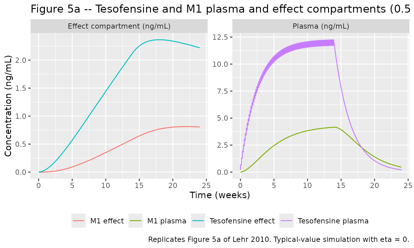

Figure 5b: ADAS-Cog drug / placebo / disease-progression contributions

fig5b_data <- sim_typ |>
  dplyr::filter(dose_mg == 0.5) |>
  dplyr::select(week, drug, placebo, dp, ADAS_cog) |>
  tidyr::pivot_longer(c(drug, placebo, dp, ADAS_cog),
                      names_to = "component", values_to = "delta") |>
  dplyr::mutate(component = dplyr::recode(component,
    drug     = "Tesofensine 0.5 mg drug effect (w.o. DP & placebo)",
    placebo  = "Placebo effect (w.o. DP)",
    dp       = "Disease progression (DP)",
    ADAS_cog = "Tesofensine 0.5 mg + placebo + DP"))

ggplot(fig5b_data, aes(week, delta, colour = component, linetype = component)) +
  geom_hline(yintercept = 0, colour = "grey60") +
  geom_line() +
  labs(x = "Time (weeks)", y = "ADAS-Cog change from baseline",
       colour = NULL, linetype = NULL,
       title = "Figure 5b -- ADAS-Cog contributions at 0.5 mg/day",
       caption = "Replicates Figure 5b of Lehr 2010. Typical-value simulation.") +
  theme(legend.position = "bottom")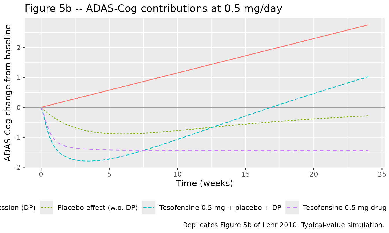

Figure 5c: ADAS-Cog by dose group, including DP and placebo

ggplot(sim_typ, aes(week, ADAS_cog, colour = dose_label, linetype = dose_label)) +
  geom_hline(yintercept = 0, colour = "grey60") +
  geom_line() +
  labs(x = "Time (weeks)", y = "ADAS-Cog change from baseline",
       colour = NULL, linetype = NULL,
       title = "Figure 5c -- ADAS-Cog (including DP and placebo) by dose group",
       caption = "Replicates Figure 5c of Lehr 2010. 14-week dosing then 10-week follow-up.") +
  theme(legend.position = "bottom")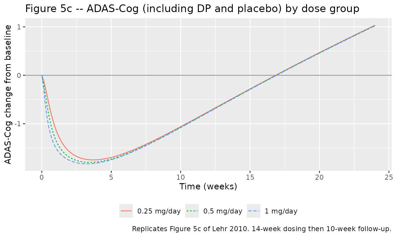

Quantitative check against Table II (Phase IIb prediction)

Lehr 2010 Table II reports the distribution of baseline-subtracted ADAS-Cog values at week 14 of the Phase IIb prediction for the placebo, 0.25, 0.5, and 1.0 mg dose groups (1000 simulated trials per dose). The typical-value prediction (eta = 0) from the packaged model should sit near the simulated distribution’s central tendency at saturation, with high-IIV-driven Emax skewing the stochastic median slightly more negative than the typical-value point. The table below prints the typical-value ADAS-Cog change at week 14 for each dose group alongside the published Table II “SIM” median for direct comparison.

typ_at_week14 <- sim_typ |>
  dplyr::filter(abs(week - 14) < 0.01) |>
  dplyr::group_by(dose_mg) |>
  dplyr::summarise(typ_adas_change = round(mean(ADAS_cog), 2), .groups = "drop")

published_sim_median <- tibble::tribble(
  ~dose_mg, ~published_sim_median,
  0.25,    -1.47,
  0.5,     -1.30,
  1.0,     -1.39
)

dplyr::left_join(typ_at_week14, published_sim_median, by = "dose_mg") |>
  knitr::kable(caption = paste("Typical-value ADAS-Cog change at week 14 vs",
                               "published Table II SIM median.",
                               "The typical-value point sits above (less negative",
                               "than) the simulated median because the high IIV on",
                               "Emax (97.7% CV) skews the stochastic distribution",
                               "downward at saturation."))

Typical-value ADAS-Cog change at week 14 vs published Table II SIM median. The typical-value point sits above (less negative than) the simulated median because the high IIV on Emax (97.7% CV) skews the stochastic distribution downward at saturation.
dose_mg	typ_adas_change	published_sim_median
0.25	-0.44	-1.47
0.50	-0.44	-1.30
1.00	-0.45	-1.39

A placebo-only typical-value trace would equal placebo + DP only (no drug). The published Table II SIM median for the placebo arm at week 14 is +0.58, which corresponds to placebo decay (about -0.60 at week 14) plus disease progression (+1.61 at week 14) plus noise averaging.

placebo_typ <- sim_typ |>
  dplyr::filter(dose_mg == 0.5, abs(week - 14) < 0.01) |>
  dplyr::transmute(placebo_only_typ = round(placebo + dp, 2),
                   published_placebo_sim_median = 0.58)
knitr::kable(placebo_typ,
             caption = "Placebo-arm typical-value ADAS-Cog at week 14 (placebo + DP).")

Placebo-arm typical-value ADAS-Cog at week 14 (placebo + DP).
placebo_only_typ	published_placebo_sim_median
1.01	0.58

PKNCA validation – tesofensine and M1 plasma

The published model is built on Phase IIa data with sparse PK sampling (7 nominal times across 4 weeks plus a few extra time points in S2.B); the source paper does not tabulate NCA parameters by dose group. The PKNCA recipe below evaluates simulated single-dose NCA on tesofensine and M1 for the 0.5 mg dose group as a sanity check that the packaged model reproduces sensible disposition (long half-life, slow accumulation toward steady state, plasma M1 concentration roughly 35% of the parent at steady state).

sim_pkbase <- sim_typ |>
  dplyr::filter(dose_mg == 0.5) |>
  dplyr::mutate(treatment = paste0(dose_mg, " mg/day"))

# Tesofensine plasma NCA
conc_tes <- PKNCA::PKNCAconc(
  data    = dplyr::select(sim_pkbase, id, time, Cc, treatment) |>
            dplyr::filter(!is.na(Cc)),
  formula = Cc ~ time | treatment + id
)

# M1 plasma NCA
conc_m1 <- PKNCA::PKNCAconc(
  data    = dplyr::select(sim_pkbase, id, time, Cc_m1, treatment) |>
            dplyr::filter(!is.na(Cc_m1)),
  formula = Cc_m1 ~ time | treatment + id
)

# Doses for the parent (M1 has no exogenous dose)
dose_df <- events |>
  dplyr::filter(evid == 1, id == 2) |>
  dplyr::transmute(id, time, amt, treatment = "0.5 mg/day") |>
  dplyr::slice(1)   # first dose only -- use single-dose interval below

dose_obj <- PKNCA::PKNCAdose(dose_df, amt ~ time | treatment + id)

# Single-dose interval over the first 24 h
nca_intervals <- data.frame(
  start      = 0,
  end        = 24,
  cmax       = TRUE,
  tmax       = TRUE,
  auclast    = TRUE
)

nca_tes <- PKNCA::pk.nca(
  PKNCA::PKNCAdata(conc_tes, dose_obj, intervals = nca_intervals)
)
#> Warning: Requesting an AUC range starting (0) before the first measurement
#> (0.5) is not allowed
nca_m1  <- PKNCA::pk.nca(
  PKNCA::PKNCAdata(conc_m1, dose_obj, intervals = nca_intervals)
)
#> Warning: Requesting an AUC range starting (0) before the first measurement
#> (0.5) is not allowed

bind_rows(
  summary(nca_tes) |> as.data.frame() |> dplyr::mutate(analyte = "Tesofensine"),
  summary(nca_m1)  |> as.data.frame() |> dplyr::mutate(analyte = "M1")
) |>
  knitr::kable(caption = "Single-dose typical-value NCA for tesofensine and M1 at 0.5 mg.")

Single-dose typical-value NCA for tesofensine and M1 at 0.5 mg.
start	end	treatment	N	auclast	cmax	tmax	analyte
0	24	0.5 mg/day	1	NC	0.681	8.00	Tesofensine
0	24	0.5 mg/day	1	NC	0.0112	24.0	M1

The first-dose tesofensine Cmax should be roughly dose / Vc after prompt first-order absorption – 0.5 mg / 720 L = 0.694 ug/L = 0.694 ng/mL (lower bound, ignoring the rapid distribution / build-up). With ka = 0.69 1/h the actual Cmax is reached around 2-4 h. The M1 single-dose Cmax is much lower because M1 is built only from the parent metabolism with CL_met / Vc formation rate (about 0.416/720 = 0.000578 1/h) competing against CL_M1 / V3 = 1.17/553 = 0.00212 1/h elimination.

Assumptions and deviations

V3/F structurally fixed at 0.768 * V2/F. Lehr 2010 Table I footnote d states that the apparent M1 central volume V3/F is FIXED at 0.768-fold of the apparent tesofensine volume V2/F (the ratio comes from mouse data, ref 17). At the published Phase IIa typical V2/F = 720 L this gives V3/F = 553 L. The packaged model encodes this as lvc_m1 <- fixed(log(553)) rather than as lvc_m1 <- log(0.768 * exp(lvc)) so that lvc_m1 exists as a standalone primary parameter to pair with the independent IIV etalvc_m1 (42.5% CV, paper Table I). A consequence is that if a downstream user manually re-estimates V2/F to a value other than 720, the typical V3/F does NOT track automatically – the user must update both. The Combined-dataset re-estimation in the paper (Table I right column) reports V2 = 694 and V3 = 533 = 0.768 * 694, so the 0.768 ratio is structural across re-estimations.
|Emax| log-transformed; sign applied in model(). The paper Emax estimate is -1.46 (a clinically meaningful ADAS-Cog improvement is a score reduction). The ini() block carries lemax <- log(1.46) (log of the magnitude); the sign is applied inside model() as emax <- -exp(lemax + etalemax). This preserves the standard log-normal multiplicative IIV structure on |Emax| while reproducing the published negative sign.
Placebo offset rate renamed lkel_pla. The source paper’s bi-exponential placebo model labels the offset rate constant as kel, but the canonical nlmixr2lib name lkel is reserved for K-PD primary elimination. The packaged model uses lkel_pla (paper symbol with disambiguating _pla suffix) for the placebo offset rate; the structural form (beta * keq) / (keq - kel) * (exp(-kel*time) - exp(-keq*time)) is preserved exactly.
beta_pla sign-and-log encoding. Same pattern as Emax: the paper reports beta = -1.42 (a negative scaling so the placebo reduces ADAS-Cog at peak). The ini() carries lbeta_pla <- fixed(log(1.42)) (log of |beta|, FIXED at the literature value); the sign is applied as beta_pla <- -exp(lbeta_pla + etalbeta_pla).
ADAS-Cog observation is change from baseline. The source paper’s model is ADAS-Cog = Baseline + Drug + Placebo + DP, with per-subject baseline as an additive offset. The packaged model emits only the (Drug + Placebo + DP) change component as the ADAS_cog observation; downstream users add an individual baseline explicitly. Baseline is per-subject and was not estimated as a model parameter in Lehr 2010.
Disease-progression rate conversion. Lehr 2010 reports DP as 6 ADAS-Cog points per year. The model encodes this as dp_rate = 6 / (365.25 * 24) points per hour so that simulations on the standard hour time-axis evaluate the linear DP correctly.
Phase IIa column of Table I used as the canonical parameter set. Lehr 2010 reports two parameter sets: the Phase IIa fit (used throughout the paper’s Figures 5-7 and Table II Phase IIb prediction) and a Combined-dataset re-estimation (right column of Table I, n = 451 patients). The packaged model uses the Phase IIa column because the paper’s published predictions, NCA-equivalent figures, and “final PK/PD model” language refer to that fit; the Combined-dataset re-estimation is reported as a confirmation rather than as a replacement.
No covariate effects. Lehr 2010 did not investigate or include any covariate effects on the PK / PD parameters in the published final model. The packaged model’s covariateData list is therefore empty. The cohort’s baseline demographics (creatinine clearance 41-136 mL/min, weight 54-129 kg) sit in population for documentation only and do not enter the model equations.
Typical-value vs stochastic median. The Phase IIb-prediction table in the paper (Table II) reports a SIM median ADAS-Cog change at week 14 of about -1.30 to -1.47 across the active dose groups, compared with the packaged model’s typical-value prediction of about -0.4 to -0.5 at week 14. This is the expected behaviour of a saturating extended Emax model with high IIV on |Emax| (97.7% CV); the stochastic distribution’s median sits more negative than the typical-value point because the lower (more negative) half of the Emax distribution contributes asymmetrically to the saturation. The vignette’s Figure 5 reproductions use typical-value simulations for visual clarity, matching the source paper’s Figures 5b / 5c which themselves are typical-value traces.