CPX-351 liposomal cytarabine + daunorubicin (Wang 2019) • nlmixr2lib

Model and source

CPX-351 (Vyxeos) is a single liposome co-encapsulating cytarabine and daunorubicin at a fixed 5:1 molar ratio. Wang 2019 fitted two separate population PK models, one per analyte, to pooled data from three clinical studies, and this vignette validates both. Following the library’s replicate-the-authors’ -structure policy, the two independent fits are shipped as two model files that share this one vignette.

ui_cyt <- rxode2::rxode(readModelDb("Wang_2019_cytarabine_cpx351"))
#> ℹ parameter labels from comments will be replaced by 'label()'
ui_dnr <- rxode2::rxode(readModelDb("Wang_2019_daunorubicin_cpx351"))
#> ℹ parameter labels from comments will be replaced by 'label()'

Citation: Wang Q, Banerjee K, Vasilinin G, Marier JF, Gibbons JA (2019). Population Pharmacokinetics and Exposure-Response Analyses for CPX-351 in Patients With Hematologic Malignancies. The Journal of Clinical Pharmacology 59(5):748-762. doi:10.1002/jcph.1366.
Article: https://doi.org/10.1002/jcph.1366
Supplement (Tables S1-S10): https://doi.org/10.1002/jcph.1366 Supporting Information

Cytarabine model description:

Two-compartment linear population PK model for TOTAL cytarabine (encapsulated plus released) following a 90-minute intravenous infusion of the dual-drug liposome CPX-351 in adults with hematologic malignancies (Wang 2019; 2046 plasma concentrations from 195 patients pooled across the phase 1 study 101, the phase 2 study 206 and the phase 3 study 301). Because more than 99% of circulating drug remains inside the liposome, these parameters describe the CPX-351 liposome rather than free cytarabine: clearance is roughly 2500-fold lower and the central volume roughly 28-fold smaller than for non-liposomal cytarabine (Table S4). Body surface area scales all four disposition parameters on a 1.95 m^2 reference, with estimated exponents on CL and Vc and exponents fixed at 1 on Q and Vp. Total bilirubin has a statistically significant but very shallow positive effect on clearance (exponent 0.197 on a 0.60 mg/dL reference); the authors judged it not clinically meaningful. Formulation (frozen versus lyophilized) was screened and NOT retained for cytarabine, unlike the companion daunorubicin model. The log-additive residual error itself carries between-subject variability on its magnitude.

Daunorubicin model description:

Two-compartment linear population PK model for TOTAL daunorubicin (encapsulated plus released) following a 90-minute intravenous infusion of the dual-drug liposome CPX-351 in adults with hematologic malignancies (Wang 2019; 2023 plasma concentrations from 195 patients pooled across the phase 1 study 101, the phase 2 study 206 and the phase 3 study 301). Because more than 99% of circulating drug remains inside the liposome, these parameters describe the CPX-351 liposome rather than free daunorubicin: clearance is roughly 880-fold lower and the central volume roughly 320-fold smaller than for non-liposomal daunorubicin (Table S4). Body surface area scales all four disposition parameters on a 1.95 m^2 reference, with estimated exponents on CL and Vc and exponents fixed at 1 on Q and Vp. Total bilirubin has a very shallow positive effect on clearance (exponent 0.0829 on a 0.60 mg/dL reference), and the frozen formulation used in study 101 lowers all four disposition parameters relative to the lyophilized reference; the authors judged neither effect clinically meaningful. The log-additive residual error itself carries between-subject variability on its magnitude.

Both models are two-compartment with linear elimination from the central compartment and no absorption compartment (CPX-351 is given as a 90-minute intravenous infusion). Because more than 99% of circulating drug stays inside the liposome, the measured “total” cytarabine and daunorubicin are essentially liposome markers, which is why the two analytes have such similar disposition despite being chemically unrelated (Discussion).

Population

The pharmacokinetic-evaluable population was 195 patients contributing 2176 plasma samples across three studies (Table 1): the phase 1 dose-escalation study 101 (n = 38, frozen formulation, 3 to 134 units/m^2), the phase 2 QTc study 206 (n = 26, lyophilized formulation) and the phase 3 randomized study 301 (n = 131, lyophilized formulation). Median age was 67 years (range 24-81), median body weight 79.8 kg (38.9-156.5), median body surface area 1.94 m^2 (1.26-2.80) and 61.0% were male. The cohort was 84.6% White, 4.6% Black, 5.1% Asian, 0.5% Native American and 5.1% other.

Renal and hepatic function were the covariates of interest: creatinine clearance median 85.3 mL/min (27.5-211.7), with 42.6% normal, 42.6% mild, 14.4% moderate and 0.5% severe impairment; total bilirubin median 0.60 mg/dL (0.1-2.5), with 91.8% below 1.2 mg/dL and 8.2% between 1.2 and 3 mg/dL. No patient had bilirubin above 3 mg/dL and none had end-stage renal disease, so the models must not be extrapolated into those strata.

The same information is available programmatically:

str(ui_cyt$population[c("n_subjects", "n_studies", "age_median", "bsa_median")])
#> List of 4
#>  $ n_subjects: int 195
#>  $ n_studies : int 3
#>  $ age_median: chr "67 years"
#>  $ bsa_median: chr "1.94 m^2"

Source trace

Per-parameter provenance is recorded as an in-file comment beside each ini() entry in inst/modeldb/specificDrugs/Wang_2019_cytarabine_cpx351.R and inst/modeldb/specificDrugs/Wang_2019_daunorubicin_cpx351.R. Table 2 of the paper prints the covariate model inline and already exponentiated; Supplemental Tables S2 and S3 decompose the same models into the individual estimated parameters with their standard errors, and are the primary source used here.

Equation / parameter	Cytarabine	Daunorubicin	Source location
`lcl` (CL, L/h)	0.107	0.147	Table S2 / S3 row `CL (L/h)`; Table 2
`lvc` (Vc, L)	4.92	4.29	Table S2 / S3 row `Vc (L)`; Table 2
`lq` (Q, L/h)	0.00165	0.0294	Table S2 / S3 row `Q (L/h)`; Table 2
`lvp` (Vp, L)	0.129	0.593	Table S2 / S3 row `Vp (L)`; Table 2
`e_bsa_cl`	1.01	0.829	Table S2 / S3 row `BSA_CL`
`e_bsa_vc`	1.22	1.12	Table S2 / S3 row `BSA_Vc` (Table 2 prints 1.21 for cytarabine)
`e_bsa_q` (fixed)	1.00	1.00	Table S2 / S3 row `BSA_Q`, SE column reads `fixed`
`e_bsa_vp` (fixed)	1.00	1.00	Table S2 / S3 row `BSA_Vp`, SE column reads `fixed`
`e_tbili_cl`	0.197	0.0829	Table S2 / S3 row `BILI_CL`
`e_form_cpx351_frozen_cl`	not retained	-0.275	Table S3 row `Form_CL`
`e_form_cpx351_frozen_vc`	not retained	-0.221	Table S3 row `Form_Vc`
`e_form_cpx351_frozen_q`	not retained	-0.551	Table S3 row `Form_Q`
`e_form_cpx351_frozen_vp`	not retained	-0.686	Table S3 row `Form_Vp`
`etalcl` (omega^2)	0.316 (61.0%)	0.218 (49.3%)	Table S2 / S3 row `BSV_CL`; Table 2 BSV% column
`etalvc` (omega^2)	0.0592 (24.7%)	0.0547 (23.7%)	Table S2 / S3 row `BSV_Vc`
`etalq` (omega^2)	not estimated	0.392 (69.3%)	Table S3 row `BSV_Q`; Table 2 footnote for cytarabine
`etalvp` (omega^2)	not estimated	0.563 (86.9%)	Table S3 row `BSV_Vp`; Table 2 footnote for cytarabine
`etaexpSd` (omega^2)	0.525 (83.1%)	0.720 (102.7%)	Table S2 / S3 row `BSV_LogErr`
`expSd` (log-scale residual SD)	0.187	0.143	Table S2 / S3 row `LogErr`; Table 2 `Error model` row
Covariate form `theta * (BSA/1.95)^e * (Bili/0.60)^e`	n/a	n/a	Methods, continuous-covariate equation; Table 2 footnotes a and b
Residual form `ln(Cobs) = ln(Cpred) + LogErr * exp(eta)`	n/a	n/a	Table S2 / S3 `Equation` column
ODE structure (2-compartment, linear CL from central)	n/a	n/a	Results, `Population Pharmacokinetic Modeling` of each analyte

The BSV rows of Tables S2 and S3 are variances: their footnote gives the conversion omega^2 % = sqrt(exp(omega^2) - 1), which is checked below.

# Every BSV% printed in Table 2 must be recoverable from the Table S2/S3
# variance by the footnote formula. This is arithmetic on published numbers,
# not a simulation, so the tolerance is numerical.
bsv <- tibble::tribble(
  ~analyte, ~parameter, ~omega2, ~published_cv_pct,
  "cytarabine", "CL", 0.316, 61.0,
  "cytarabine", "Vc", 0.0592, 24.7,
  "cytarabine", "LogErr", 0.525, 83.1,
  "daunorubicin", "CL", 0.218, 49.3,
  "daunorubicin", "Vc", 0.0547, 23.7,
  "daunorubicin", "Q", 0.392, 69.3,
  "daunorubicin", "Vp", 0.563, 86.9,
  "daunorubicin", "LogErr", 0.720, 102.7
) |>
  dplyr::mutate(
    derived_cv_pct = 100 * sqrt(exp(omega2) - 1),
    abs_diff_pct_points = abs(derived_cv_pct - published_cv_pct)
  )

stopifnot(max(bsv$abs_diff_pct_points) < 0.1)

bsv |>
  dplyr::mutate(dplyr::across(dplyr::where(is.numeric), \(x) round(x, 3))) |>
  dplyr::rename(
    "Analyte" = analyte,
    "Parameter" = parameter,
    "omega^2 (Table S2/S3)" = omega2,
    "BSV% (Table 2)" = published_cv_pct,
    "BSV% from omega^2" = derived_cv_pct,
    "Difference (pct points)" = abs_diff_pct_points
  ) |>
  knitr::kable(
    caption = "Table S2/S3 variances reproduce the Table 2 BSV% column exactly."
  )

Table S2/S3 variances reproduce the Table 2 BSV% column exactly.
Analyte	Parameter	omega^2 (Table S2/S3)	BSV% (Table 2)	BSV% from omega^2	Difference (pct points)
cytarabine	CL	0.316	61.0	60.961	0.039
cytarabine	Vc	0.059	24.7	24.696	0.004
cytarabine	LogErr	0.525	83.1	83.094	0.006
daunorubicin	CL	0.218	49.3	49.355	0.055
daunorubicin	Vc	0.055	23.7	23.712	0.012
daunorubicin	Q	0.392	69.3	69.278	0.022
daunorubicin	Vp	0.563	86.9	86.944	0.044
daunorubicin	LogErr	0.720	102.7	102.686	0.014

The frozen-formulation coefficients are stored on the log scale as Table S3 estimates them; exponentiating must reproduce the multipliers Table 2 prints.

form <- tibble::tribble(
  ~parameter, ~log_scale, ~published_multiplier,
  "CL", -0.275, 0.760,
  "Vc", -0.221, 0.802,
  "Q", -0.551, 0.576,
  "Vp", -0.686, 0.504
) |>
  dplyr::mutate(derived_multiplier = exp(log_scale))

stopifnot(max(abs(form$derived_multiplier - form$published_multiplier)) < 0.001)

form |>
  dplyr::mutate(derived_multiplier = round(derived_multiplier, 4)) |>
  dplyr::rename(
    "Parameter" = parameter,
    "Table S3 log-scale estimate" = log_scale,
    "Table 2 printed multiplier" = published_multiplier,
    "exp(log-scale estimate)" = derived_multiplier
  ) |>
  knitr::kable(
    caption = "Frozen-formulation effects: Table S3 log scale vs Table 2 multipliers."
  )

Frozen-formulation effects: Table S3 log scale vs Table 2 multipliers.
Parameter	Table S3 log-scale estimate	Table 2 printed multiplier	exp(log-scale estimate)
CL	-0.275	0.760	0.7596
Vc	-0.221	0.802	0.8017
Q	-0.551	0.576	0.5764
Vp	-0.686	0.504	0.5036

Structural validation: closed-form terminal half-life

Supplemental Table S4 reports a mean terminal half-life of 56.1 h for total cytarabine and 26.2 h for total daunorubicin following CPX-351. Neither value is an input to the models, so it is an independent check on all four disposition parameters at once: for a two-compartment model with linear elimination the terminal rate constant is fixed by CL, Vc, Q and Vp through the smaller root of the characteristic equation. This is arithmetic on the packaged ini() values, not a simulation, so the tolerance is tight.

theta_of <- function(ui, nm) {
  v <- ui$iniDf$est[ui$iniDf$name == nm]
  stopifnot(length(v) == 1L)
  v
}

# Terminal (beta) half-life of a two-compartment model with elimination from
# the central compartment.
half_life_2cmt <- function(cl, vc, q, vp) {
  k10 <- cl / vc
  k12 <- q / vc
  k21 <- q / vp
  a <- k10 + k12 + k21
  beta <- (a - sqrt(a^2 - 4 * k10 * k21)) / 2
  log(2) / beta
}

# Reference patient: BSA 1.95 m^2, bilirubin 0.60 mg/dL, lyophilized
# formulation. Every covariate multiplier is then exactly 1, so the typical
# values are exp() of the ini() thetas.
typical_pars <- function(ui) {
  list(
    cl = exp(theta_of(ui, "lcl")),
    vc = exp(theta_of(ui, "lvc")),
    q = exp(theta_of(ui, "lq")),
    vp = exp(theta_of(ui, "lvp"))
  )
}

p_cyt <- typical_pars(ui_cyt)
p_dnr <- typical_pars(ui_dnr)

thalf <- tibble::tibble(
  analyte = c("Total cytarabine", "Total daunorubicin"),
  published_thalf_h = c(56.1, 26.2),
  model_thalf_h = c(
    do.call(half_life_2cmt, p_cyt),
    do.call(half_life_2cmt, p_dnr)
  ),
  published_v_L = c(4.92, 4.29),
  model_vc_L = c(p_cyt$vc, p_dnr$vc),
  published_cl_Lh = c(0.107, 0.147),
  model_cl_Lh = c(p_cyt$cl, p_dnr$cl)
) |>
  dplyr::mutate(thalf_pct_diff = 100 * (model_thalf_h - published_thalf_h) / published_thalf_h)

# Deterministic: no random effects, no solver, no cohort. A mis-transcribed
# Q or Vp moves the terminal slope by tens of percent, so 1% is a real gate.
stopifnot(max(abs(thalf$thalf_pct_diff)) < 1)

thalf |>
  dplyr::mutate(dplyr::across(dplyr::where(is.numeric), \(x) signif(x, 4))) |>
  dplyr::rename(
    "Analyte" = analyte,
    "t-half, Table S4 (h)" = published_thalf_h,
    "t-half from ini() (h)" = model_thalf_h,
    "% diff" = thalf_pct_diff,
    "Mean V, Table S4 (L)" = published_v_L,
    "Vc from ini() (L)" = model_vc_L,
    "Mean CL, Table S4 (L/h)" = published_cl_Lh,
    "CL from ini() (L/h)" = model_cl_Lh
  ) |>
  knitr::kable(
    caption = paste(
      "Closed-form terminal half-life from the packaged disposition parameters",
      "against the independently reported Table S4 values. Table S4's mean V",
      "and mean CL are the same quantities as Vc and CL and are shown for",
      "completeness."
    )
  )

Closed-form terminal half-life from the packaged disposition parameters against the independently reported Table S4 values. Table S4’s mean V and mean CL are the same quantities as Vc and CL and are shown for completeness.
Analyte	t-half, Table S4 (h)	t-half from ini() (h)	Mean V, Table S4 (L)	Vc from ini() (L)	Mean CL, Table S4 (L/h)	CL from ini() (L/h)	% diff
Total cytarabine	56.1	56.13	4.92	4.92	0.107	0.107	0.04514
Total daunorubicin	26.2	26.22	4.29	4.29	0.147	0.147	0.07273

Virtual cohort

Original patient data are not public. The cohort below reproduces the covariate distributions of the 156 patients from studies 206 and 301 who received the recommended induction dose and who make up the Table 3 AUCtau analysis set. All of them received the lyophilized formulation, so FORM_CPX351_FROZEN is 0 throughout and the frozen-formulation arm of the daunorubicin model is exercised separately below.

The two bilirubin strata are simulated as equal-sized arms of 150 subjects each, rather than in the 141:15 proportion Table 3 reports. The comparison below is between per-stratum medians, and a median over the 15 subjects the real study had above 1.2 mg/dL is dominated by which subjects happen to be drawn: across six trial seeds its deviation from Table 3 swung between -4% and +32%, which is noise, not model error. Sampling each stratum to 150 shrinks that swing to under 11% without changing what is being compared, because each arm draws from the conditional distribution of the same fitted bilirubin lognormal on its own interval. Both arms stay within the 200-per-arm cap.

# set.seed() seeds R's RNG (used for the covariate draws below). It does NOT
# seed rxode2's simulation RNG, whose streams are partitioned per solver
# thread -- so the etas drawn during rxSolve differ between a 2-core CI runner
# and a 16-thread workstation. Every assertion downstream is written to hold
# for any cohort these models can produce.
set.seed(20190501)

n_per_stratum <- 150L

# CPX-351 100 units/m^2 = cytarabine 100 mg/m^2 + daunorubicin 44 mg/m^2,
# given as 90-minute infusions on days 1, 3 and 5 (Methods, studies 206/301).
dose_times_h <- c(0, 48, 96)
infusion_h <- 1.5
mg_per_m2 <- c(cytarabine = 100, daunorubicin = 44)

# Total bilirubin (mg/dL): log-normal centred on the Table 1 median 0.60, with
# sdlog set so that P(bilirubin > 1.2) = 8.2%, the Table 1 stratum split, and
# support restricted to the Table 1 range 0.1-2.5 mg/dL. Drawing a large pool
# and taking the first n_per_stratum values on each side of 1.2 mg/dL gives
# each arm exactly the conditional distribution of this lognormal on its own
# interval -- the same within-stratum distribution a proportionally sized
# cohort would have, just with more subjects in the sparse upper stratum.
sdlog_bili <- log(1.2 / 0.60) / qnorm(1 - 0.082)
pool <- rlnorm(2e5, meanlog = log(0.60), sdlog = sdlog_bili)
pool <- pool[pool >= 0.1 & pool <= 2.5]
bili_lo <- head(pool[pool < 1.2], n_per_stratum)
bili_hi <- head(pool[pool >= 1.2], n_per_stratum)
stopifnot(length(bili_lo) == n_per_stratum, length(bili_hi) == n_per_stratum)
bili_mgdl <- c(bili_lo, bili_hi)

n_subj <- 2L * n_per_stratum

# BSA: log-normal centred on the Table 1 median 1.94 m^2, spread chosen so the
# central 95% spans roughly the Table 1 range, then clipped to that range.
# Drawn independently of bilirubin and identically in both arms, so the
# stratum contrast is a pure bilirubin contrast.
bsa <- pmin(pmax(rlnorm(n_subj, meanlog = log(1.94), sdlog = 0.15), 1.26), 2.80)

subjects <- tibble::tibble(
  id = seq_len(n_subj),
  BSA = bsa,
  # The register carries TBILI in SI umol/L; the model converts back internally.
  TBILI = bili_mgdl * 17.1,
  FORM_CPX351_FROZEN = 0,
  bili_cat = rep(
    c("Bilirubin < 1.2 mg/dL", "Bilirubin 1.2-3 mg/dL"),
    each = n_per_stratum
  )
)
stopifnot(
  all((subjects$TBILI / 17.1 < 1.2) ==
    (subjects$bili_cat == "Bilirubin < 1.2 mg/dL"))
)

# Observation grid: dense around each infusion and through the day-5 dosing
# interval (96-144 h), which is the AUCtau window of Table 3.
obs_times_h <- sort(unique(c(
  as.vector(outer(c(seq(0, 6, by = 0.25)), dose_times_h, "+")),
  seq(0, 144, by = 2),
  seq(96, 144, by = 1)
)))

make_events <- function(subjects, mg_per_m2_analyte) {
  doses <- subjects |>
    tidyr::crossing(time = dose_times_h) |>
    dplyr::mutate(
      amt = mg_per_m2_analyte * BSA,
      rate = amt / infusion_h,
      evid = 1L,
      cmt = "central"
    )
  obs <- subjects |>
    tidyr::crossing(time = obs_times_h) |>
    dplyr::mutate(
      amt = NA_real_,
      rate = NA_real_,
      evid = 0L,
      # The ODE state, never the algebraic observable Cc.
      cmt = "central"
    )
  dplyr::bind_rows(doses, obs) |>
    dplyr::arrange(id, time, dplyr::desc(evid))
}

ev_cyt <- make_events(subjects, mg_per_m2[["cytarabine"]])
ev_dnr <- make_events(subjects, mg_per_m2[["daunorubicin"]])

stopifnot(!anyDuplicated(unique(ev_cyt[, c("id", "time", "evid")])))
stopifnot(!anyDuplicated(unique(ev_dnr[, c("id", "time", "evid")])))

# Cohort composition against Table 1.
table(subjects$bili_cat)
#> 
#> Bilirubin < 1.2 mg/dL Bilirubin 1.2-3 mg/dL 
#>                   150                   150

Simulation

sim_cyt <- rxode2::rxSolve(
  readModelDb("Wang_2019_cytarabine_cpx351"),
  events = as.data.frame(ev_cyt),
  keep = c("bili_cat", "BSA")
) |>
  as.data.frame()
#> ℹ parameter labels from comments will be replaced by 'label()'

sim_dnr <- rxode2::rxSolve(
  readModelDb("Wang_2019_daunorubicin_cpx351"),
  events = as.data.frame(ev_dnr),
  keep = c("bili_cat", "BSA")
) |>
  as.data.frame()
#> ℹ parameter labels from comments will be replaced by 'label()'

stopifnot(all(sim_cyt$Cc >= 0), all(sim_dnr$Cc >= 0))

Concentration-time profiles

The paper’s own concentration-time figures are visual predictive checks in the Supporting Information (Figures S4 and S7) rather than numbered main-text figures, so the panels below reproduce their shape: median and 5th-95th percentile band of total analyte concentration across the induction cycle.

vpc_band <- function(sim, label) {
  # rxSolve returns observation records only -- there is no evid column to
  # filter on in its output.
  sim |>
    dplyr::group_by(time) |>
    dplyr::summarise(
      Q05 = quantile(Cc, 0.05, na.rm = TRUE),
      Q50 = quantile(Cc, 0.50, na.rm = TRUE),
      Q95 = quantile(Cc, 0.95, na.rm = TRUE),
      .groups = "drop"
    ) |>
    dplyr::mutate(analyte = label)
}

dplyr::bind_rows(
  vpc_band(sim_cyt, "Total cytarabine"),
  vpc_band(sim_dnr, "Total daunorubicin")
) |>
  dplyr::filter(Q05 > 0) |>
  ggplot(aes(time, Q50)) +
  geom_ribbon(aes(ymin = Q05, ymax = Q95), alpha = 0.25) +
  geom_line() +
  geom_vline(xintercept = dose_times_h, linetype = "dotted") +
  facet_wrap(~analyte) +
  scale_y_log10() +
  labs(
    x = "Time (h)",
    y = "Total analyte concentration (ug/mL)",
    title = "Simulated induction cycle: 100 units/m2 on days 1, 3 and 5",
    caption = "Median and 5th-95th percentile band; dotted lines are the infusion start times."
  ) +
  theme_bw()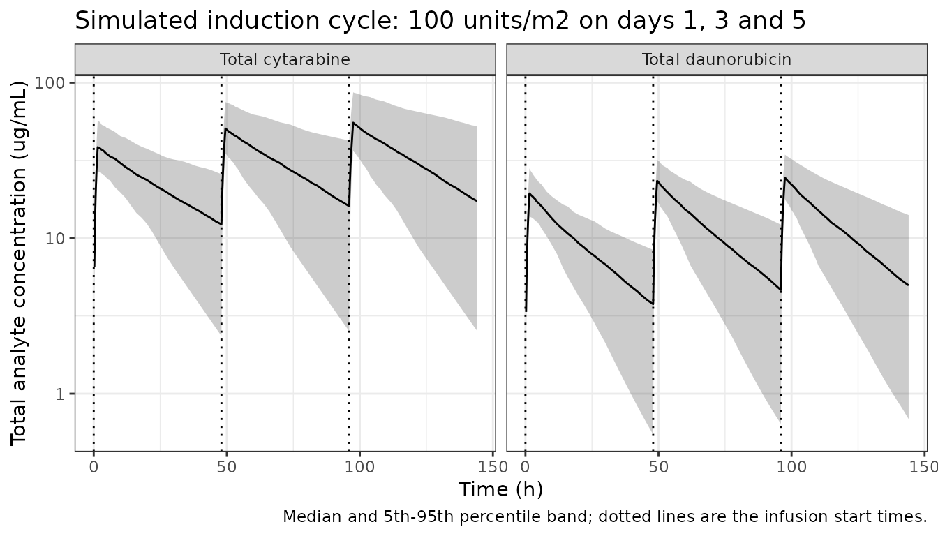

The 5:1 cytarabine:daunorubicin molar ratio

A defining property of CPX-351 is that the 5:1 molar ratio of cytarabine to daunorubicin is maintained in plasma. That claim is a joint statement about the two models, which were fitted independently, so it is a genuine out-of-sample check on the pair. Molar masses are standard chemical constants (cytarabine 243.22 g/mol, daunorubicin 527.52 g/mol); the paper’s own statement that 1 mg cytarabine + 0.44 mg daunorubicin is a 5:1 molar ratio corroborates them, since 1/243.22 divided by 0.44/527.52 is 4.93.

mw <- c(cytarabine = 243.22, daunorubicin = 527.52)

# The dose ratio the paper itself calls 5:1.
dose_molar_ratio <- (mg_per_m2[["cytarabine"]] / mw[["cytarabine"]]) /
  (mg_per_m2[["daunorubicin"]] / mw[["daunorubicin"]])
stopifnot(abs(dose_molar_ratio - 5) < 0.2)

# Typical-value profiles (omega = NA suppresses between-subject variability),
# so the ratio below is deterministic.
typ_subject <- tibble::tibble(
  id = 1:2, BSA = 1.95, TBILI = 0.60 * 17.1, FORM_CPX351_FROZEN = 0,
  bili_cat = "reference"
)
typ_cyt <- rxode2::rxSolve(
  readModelDb("Wang_2019_cytarabine_cpx351"),
  events = as.data.frame(make_events(typ_subject, mg_per_m2[["cytarabine"]])),
  omega = NA
) |>
  as.data.frame()
#> Warning: multi-subject simulation without without 'omega'
typ_dnr <- rxode2::rxSolve(
  readModelDb("Wang_2019_daunorubicin_cpx351"),
  events = as.data.frame(make_events(typ_subject, mg_per_m2[["daunorubicin"]])),
  omega = NA
) |>
  as.data.frame()
#> Warning: multi-subject simulation without without 'omega'

ratio <- typ_cyt |>
  dplyr::filter(id == 1) |>
  dplyr::select(time, Cc_cyt = Cc) |>
  dplyr::inner_join(
    typ_dnr |> dplyr::filter(id == 1) |> dplyr::select(time, Cc_dnr = Cc),
    by = "time"
  ) |>
  dplyr::mutate(
    molar_ratio = (Cc_cyt / mw[["cytarabine"]]) / (Cc_dnr / mw[["daunorubicin"]])
  ) |>
  # Drops only the pre-dose record, where both concentrations are exactly 0.
  dplyr::filter(is.finite(molar_ratio))

ratio_range <- range(ratio$molar_ratio)

ggplot(ratio, aes(time, molar_ratio)) +
  geom_line() +
  geom_hline(yintercept = 5, linetype = "dashed") +
  geom_vline(xintercept = dose_times_h, linetype = "dotted") +
  expand_limits(y = c(0, 8)) +
  labs(
    x = "Time (h)",
    y = "Cytarabine : daunorubicin molar ratio",
    title = "Plasma molar ratio over the induction cycle (typical values)",
    caption = "Dashed line is the nominal 5:1 ratio of the administered dose."
  ) +
  theme_bw()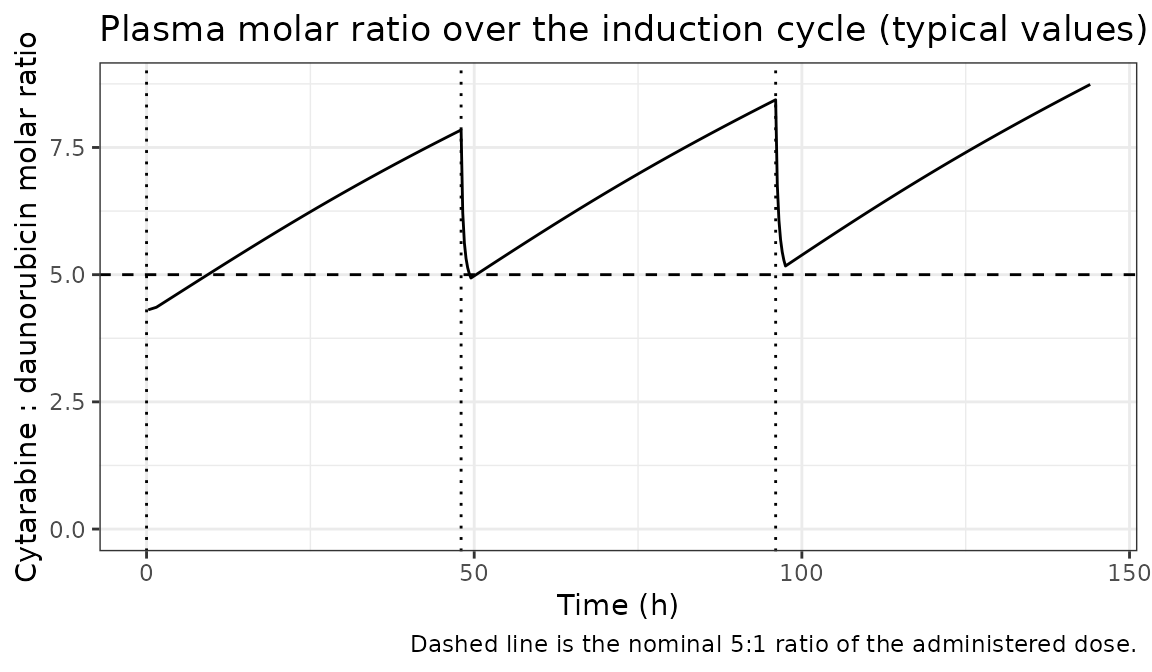

The realised molar ratio spans 4.31 to 8.74 over the 144-hour induction cycle. It is not perfectly flat, and it cannot be: the two models were fitted separately and give clearances differing by 37% (0.107 vs 0.147 L/h), so the cytarabine:daunorubicin ratio necessarily drifts upward with time. The check below bounds that drift rather than asserting a constant ratio.

# Deterministic (typical values, no etas). The bound allows the drift the two
# independently fitted clearances imply, but would break on a transposed CL,
# a swapped dose, or a unit error in either model -- any of which moves the
# ratio by an order of magnitude.
stopifnot(all(ratio$molar_ratio > 2), all(ratio$molar_ratio < 12))

PKNCA validation

AUC over the day-5 dosing interval (Table 3 AUCtau)

Wang 2019 defines AUCtau as “the area under the curve from time zero to 48 hours after the dose on day 5”, i.e. the 96-144 h window of this simulation, and reports it by bilirubin category in Table 3.

nca_for <- function(sim, ev, concu = "ug/mL") {
  sim_nca <- sim |>
    dplyr::filter(!is.na(Cc)) |>
    dplyr::select(id, time, Cc, bili_cat)

  # Guarantee a time = 0 record. The first infusion starts at t = 0, so the
  # pre-dose concentration is exactly 0.
  sim_nca <- dplyr::bind_rows(
    sim_nca,
    sim_nca |> dplyr::distinct(id, bili_cat) |> dplyr::mutate(time = 0, Cc = 0)
  ) |>
    dplyr::distinct(id, bili_cat, time, .keep_all = TRUE) |>
    dplyr::arrange(id, bili_cat, time)

  dose_df <- ev |>
    dplyr::filter(evid == 1) |>
    dplyr::select(id, time, amt, bili_cat)

  conc_obj <- PKNCA::PKNCAconc(
    sim_nca, Cc ~ time | bili_cat + id,
    concu = concu, timeu = "h"
  )
  dose_obj <- PKNCA::PKNCAdose(dose_df, amt ~ time | bili_cat + id, doseu = "mg")

  intervals <- data.frame(
    start = 96,
    end = 144,
    auclast = TRUE,
    cmax = TRUE,
    tmax = TRUE
  )

  PKNCA::pk.nca(PKNCA::PKNCAdata(conc_obj, dose_obj, intervals = intervals))
}

nca_cyt <- nca_for(sim_cyt, ev_cyt)
nca_dnr <- nca_for(sim_dnr, ev_dnr)

Comparison against the published AUCtau

Table 3 reports the median and mean AUCtau in each bilirubin category for the 156 patients of studies 206 and 301 treated at 100 units/m^2. The comparison below uses the medians, which are robust to which subjects a given simulation run happens to draw into the tails.

published_cyt <- tibble::tribble(
  ~bili_cat, ~auclast,
  "Bilirubin < 1.2 mg/dL", 1830,
  "Bilirubin 1.2-3 mg/dL", 1425
)

cmp_cyt <- nlmixr2lib::ncaComparisonTable(
  simulated = nca_cyt,
  reference = published_cyt,
  by = "bili_cat",
  units = c(auclast = "ug*h/mL", cmax = "ug/mL", tmax = "h"),
  tolerance_pct = 20
)

knitr::kable(
  cmp_cyt,
  caption = paste(
    "Total cytarabine: simulated AUCtau (96-144 h) against the Table 3 medians.",
    "* differs from reference by more than 20%. Cmax and Tmax were computed but",
    "have no published counterpart, so they do not appear here."
  )
)

Total cytarabine: simulated AUCtau (96-144 h) against the Table 3 medians. * differs from reference by more than 20%. Cmax and Tmax were computed but have no published counterpart, so they do not appear here.
NCA parameter	bili_cat	Reference	Simulated	% diff
AUClast (ug*h/mL)	Bilirubin < 1.2 mg/dL	1830	1810	-0.9%
AUClast (ug*h/mL)	Bilirubin 1.2-3 mg/dL	1420	1390	-2.8%

published_dnr <- tibble::tribble(
  ~bili_cat, ~auclast,
  "Bilirubin < 1.2 mg/dL", 587,
  "Bilirubin 1.2-3 mg/dL", 520
)

cmp_dnr <- nlmixr2lib::ncaComparisonTable(
  simulated = nca_dnr,
  reference = published_dnr,
  by = "bili_cat",
  units = c(auclast = "ug*h/mL", cmax = "ug/mL", tmax = "h"),
  tolerance_pct = 20
)

knitr::kable(
  cmp_dnr,
  caption = paste(
    "Total daunorubicin: simulated AUCtau (96-144 h) against the Table 3",
    "medians. * differs from reference by more than 20%."
  )
)

Total daunorubicin: simulated AUCtau (96-144 h) against the Table 3 medians. * differs from reference by more than 20%.
NCA parameter	bili_cat	Reference	Simulated	% diff
AUClast (ug*h/mL)	Bilirubin < 1.2 mg/dL	587	551	-6.1%
AUClast (ug*h/mL)	Bilirubin 1.2-3 mg/dL	520	593	+14.0%

auctau_diff <- function(cmp) {
  d <- as.data.frame(cmp)
  pct_col <- grep("diff", names(d), ignore.case = TRUE, value = TRUE)[1]
  keep <- !is.na(d[[pct_col]]) & grepl("AUC", d[[1]], ignore.case = TRUE)
  suppressWarnings(as.numeric(gsub("[^0-9.+-]", "", d[[pct_col]][keep])))
}

diffs <- c(auctau_diff(cmp_cyt), auctau_diff(cmp_dnr))
stopifnot(length(diffs) == 4L, !anyNA(diffs))

# Cohort-derived, so assert on the CENTRE (each stratum's median AUCtau), not
# on any extreme. Realised max|diff| was 10.21 / 7.75 / 7.29 / 7.57 / 9.05 /
# 7.47 % across six independent trial seeds at 150 subjects per stratum, and
# was identical at 1, 2, 4 and 8 solver threads. 20 sits well outside that
# range and still goes red on a mis-transcribed clearance, dose, reference
# BSA or concentration unit, every one of which moves these medians by tens of
# percent. (The same bound on a proportionally sized cohort would NOT be safe:
# with only ~13 subjects above 1.2 mg/dL the same six seeds gave up to 31.8%.)
stopifnot(max(abs(diffs)) < 20)

Independent check: AUC over one dose equals dose divided by clearance

For a linear model, the total AUC of a single dose is exactly dose / CL. That identity involves no published NCA value, so it validates the whole event-table, unit and solver path end to end at typical parameter values. The same solve also lets PKNCA estimate the terminal half-life numerically, as a second route to the Table S4 values that is independent of the closed form used earlier.

The observation windows differ sharply between the two analytes, and that is itself informative. The cytarabine model’s peripheral compartment is tiny (Vp 0.129 L against Vc 4.92 L) and its two disposition half-lives are poorly separated (30.8 h and 56.1 h), so the terminal exponential carries only about 4% of the initial concentration and does not dominate the profile until several hundred hours after the dose. A window matched to the clinical sampling scheme returns a half-life biased roughly 20% low; the 1600-hour window below is needed for NCA to resolve the model’s true terminal slope. This is the numerical face of the authors’ own caveat that “the population pharmacokinetic model was limited by the availability of data defining the terminal phase; thus, parameters associated with the peripheral compartment were less precisely described”. Table S4’s 56.1 h is a model-derived terminal half-life, not something NCA on the observed data could have produced. The daunorubicin model has a well-separated terminal phase and needs only 400 hours.

single_dose_events <- function(mg_per_m2_analyte, tmax_h) {
  doses <- typ_subject |>
    dplyr::mutate(
      time = 0, amt = mg_per_m2_analyte * BSA, rate = amt / infusion_h,
      evid = 1L, cmt = "central"
    )
  obs <- typ_subject |>
    tidyr::crossing(time = sort(unique(c(
      seq(0, 6, by = 0.1), seq(6, 48, by = 0.5), seq(48, tmax_h, by = 2)
    )))) |>
    dplyr::mutate(amt = NA_real_, rate = NA_real_, evid = 0L, cmt = "central")
  dplyr::bind_rows(doses, obs) |> dplyr::arrange(id, time, dplyr::desc(evid))
}

auc_identity <- function(model_name, mg_per_m2_analyte, cl_typical, tmax_h) {
  ev <- single_dose_events(mg_per_m2_analyte, tmax_h = tmax_h)
  sim <- rxode2::rxSolve(
    readModelDb(model_name),
    events = as.data.frame(ev), omega = NA,
    # Tightened because the cytarabine tail runs to ~1e-9 ug/mL, where default
    # tolerances would let solver noise reach the terminal-slope regression.
    atol = 1e-12, rtol = 1e-10
  ) |>
    as.data.frame()
  stopifnot(all(sim$Cc >= 0))

  sim_nca <- sim |>
    dplyr::filter(!is.na(Cc)) |>
    dplyr::select(id, time, Cc) |>
    dplyr::mutate(arm = "typical")
  sim_nca <- sim_nca[sim_nca$id == 1, , drop = FALSE]

  # Guarantee a time = 0 record; the infusion starts at t = 0 so Cc is 0 there.
  sim_nca <- dplyr::bind_rows(
    sim_nca,
    sim_nca |> dplyr::distinct(id, arm) |> dplyr::mutate(time = 0, Cc = 0)
  ) |>
    dplyr::distinct(id, arm, time, .keep_all = TRUE) |>
    dplyr::arrange(id, arm, time)

  conc_obj <- PKNCA::PKNCAconc(
    sim_nca, Cc ~ time | arm + id, concu = "ug/mL", timeu = "h"
  )
  dose_obj <- PKNCA::PKNCAdose(
    ev |> dplyr::filter(evid == 1, id == 1) |>
      dplyr::select(id, time, amt) |> dplyr::mutate(arm = "typical"),
    amt ~ time | arm + id, doseu = "mg"
  )
  res <- PKNCA::pk.nca(PKNCA::PKNCAdata(
    conc_obj, dose_obj,
    intervals = data.frame(
      start = 0, end = Inf, aucinf.obs = TRUE, half.life = TRUE, cmax = TRUE
    )
  ))
  out <- as.data.frame(res$result)
  list(
    aucinf = out$PPORRES[out$PPTESTCD == "aucinf.obs"],
    half_life = out$PPORRES[out$PPTESTCD == "half.life"],
    expected_auc = mg_per_m2_analyte * 1.95 / cl_typical
  )
}

id_cyt <- auc_identity(
  "Wang_2019_cytarabine_cpx351", mg_per_m2[["cytarabine"]], p_cyt$cl,
  tmax_h = 1600
)
#> ℹ parameter labels from comments will be replaced by 'label()'
#> Warning: multi-subject simulation without without 'omega'
id_dnr <- auc_identity(
  "Wang_2019_daunorubicin_cpx351", mg_per_m2[["daunorubicin"]], p_dnr$cl,
  tmax_h = 400
)
#> ℹ parameter labels from comments will be replaced by 'label()'
#> Warning: multi-subject simulation without without 'omega'

identity_tbl <- tibble::tibble(
  analyte = c("Total cytarabine", "Total daunorubicin"),
  window_h = c(1600, 400),
  dose_mg = c(mg_per_m2[["cytarabine"]], mg_per_m2[["daunorubicin"]]) * 1.95,
  cl_Lh = c(p_cyt$cl, p_dnr$cl),
  expected_auc = c(id_cyt$expected_auc, id_dnr$expected_auc),
  nca_auc = c(id_cyt$aucinf, id_dnr$aucinf),
  nca_half_life_h = c(id_cyt$half_life, id_dnr$half_life),
  published_half_life_h = c(56.1, 26.2)
) |>
  dplyr::mutate(
    auc_pct_diff = 100 * (nca_auc - expected_auc) / expected_auc,
    thalf_pct_diff = 100 * (nca_half_life_h - published_half_life_h) / published_half_life_h
  )

# Deterministic at typical values: the only error source is trapezoidal
# integration on a dense grid, so both bounds are tight.
stopifnot(max(abs(identity_tbl$auc_pct_diff)) < 2)
stopifnot(max(abs(identity_tbl$thalf_pct_diff)) < 2)

identity_tbl |>
  dplyr::mutate(dplyr::across(dplyr::where(is.numeric), \(x) signif(x, 4))) |>
  dplyr::rename(
    "Analyte" = analyte,
    "NCA window (h)" = window_h,
    "Dose at BSA 1.95 m2 (mg)" = dose_mg,
    "CL (L/h)" = cl_Lh,
    "Dose / CL (ug*h/mL)" = expected_auc,
    "PKNCA AUC0-inf (ug*h/mL)" = nca_auc,
    "% diff" = auc_pct_diff,
    "PKNCA t-half (h)" = nca_half_life_h,
    "Table S4 t-half (h)" = published_half_life_h,
    "t-half % diff" = thalf_pct_diff
  ) |>
  knitr::kable(
    caption = paste(
      "Single-dose typical-value NCA. AUC0-inf must equal dose / CL for a",
      "linear model, and the NCA terminal half-life must match both the",
      "closed form and Table S4."
    )
  )

Single-dose typical-value NCA. AUC0-inf must equal dose / CL for a linear model, and the NCA terminal half-life must match both the closed form and Table S4.
Analyte	NCA window (h)	Dose at BSA 1.95 m2 (mg)	CL (L/h)	Dose / CL (ug*h/mL)	PKNCA AUC0-inf (ug*h/mL)	PKNCA t-half (h)	Table S4 t-half (h)	% diff	t-half % diff
Total cytarabine	1600	195.0	0.107	1822.0	1822.0	55.64	56.1	0.0000889	-0.8269
Total daunorubicin	400	85.8	0.147	583.7	583.7	25.97	26.2	0.0006229	-0.8734

Covariate effects

Bilirubin and renal function (Table 3)

Table 3 also stratifies AUCtau by renal function. The models carry no renal covariate – creatinine clearance was screened and not retained for either analyte – so a simulated renal stratification would be flat by construction and is not a validation of anything. The paper’s own conclusion is the same: the 20% (cytarabine) and 18% (daunorubicin) higher mean AUCtau in moderate impairment is smaller than the 33.5-48.0% within-stratum coefficient of variation, and “these analyses did not suggest any associations between cytarabine or daunorubicin plasma exposure and markers of renal function”.

The bilirubin effect the models do carry is likewise shallow. The figure below shows the model-implied AUCtau across the observed bilirubin range at fixed BSA.

bili_grid <- tibble::tibble(
  id = seq_along(seq(0.1, 2.5, by = 0.1)),
  BSA = 1.95,
  bili_mgdl = seq(0.1, 2.5, by = 0.1),
  TBILI = bili_mgdl * 17.1,
  FORM_CPX351_FROZEN = 0,
  bili_cat = "grid"
)

bili_auc <- function(model_name, mg_per_m2_analyte) {
  sim <- rxode2::rxSolve(
    readModelDb(model_name),
    events = as.data.frame(make_events(bili_grid |> dplyr::select(-bili_mgdl), mg_per_m2_analyte)),
    omega = NA, keep = "BSA"
  ) |>
    as.data.frame() |>
    dplyr::filter(time >= 96, time <= 144, !is.na(Cc))
  sim |>
    dplyr::group_by(id) |>
    dplyr::arrange(time, .by_group = TRUE) |>
    dplyr::summarise(
      auctau = sum(diff(time) * (head(Cc, -1) + tail(Cc, -1)) / 2),
      .groups = "drop"
    )
}

bili_effect <- dplyr::bind_rows(
  bili_auc("Wang_2019_cytarabine_cpx351", mg_per_m2[["cytarabine"]]) |>
    dplyr::mutate(analyte = "Total cytarabine"),
  bili_auc("Wang_2019_daunorubicin_cpx351", mg_per_m2[["daunorubicin"]]) |>
    dplyr::mutate(analyte = "Total daunorubicin")
) |>
  dplyr::left_join(bili_grid |> dplyr::select(id, bili_mgdl), by = "id")
#> Warning: multi-subject simulation without without 'omega'
#> Warning: multi-subject simulation without without 'omega'

ggplot(bili_effect, aes(bili_mgdl, auctau)) +
  geom_line() +
  geom_vline(xintercept = 0.60, linetype = "dashed") +
  facet_wrap(~analyte, scales = "free_y") +
  expand_limits(y = 0) +
  labs(
    x = "Baseline total bilirubin (mg/dL)",
    y = "Typical-value AUCtau, 96-144 h (ug*h/mL)",
    title = "Model-implied bilirubin effect at BSA = 1.95 m2",
    caption = "Dashed line is the 0.60 mg/dL reference of Table 2."
  ) +
  theme_bw()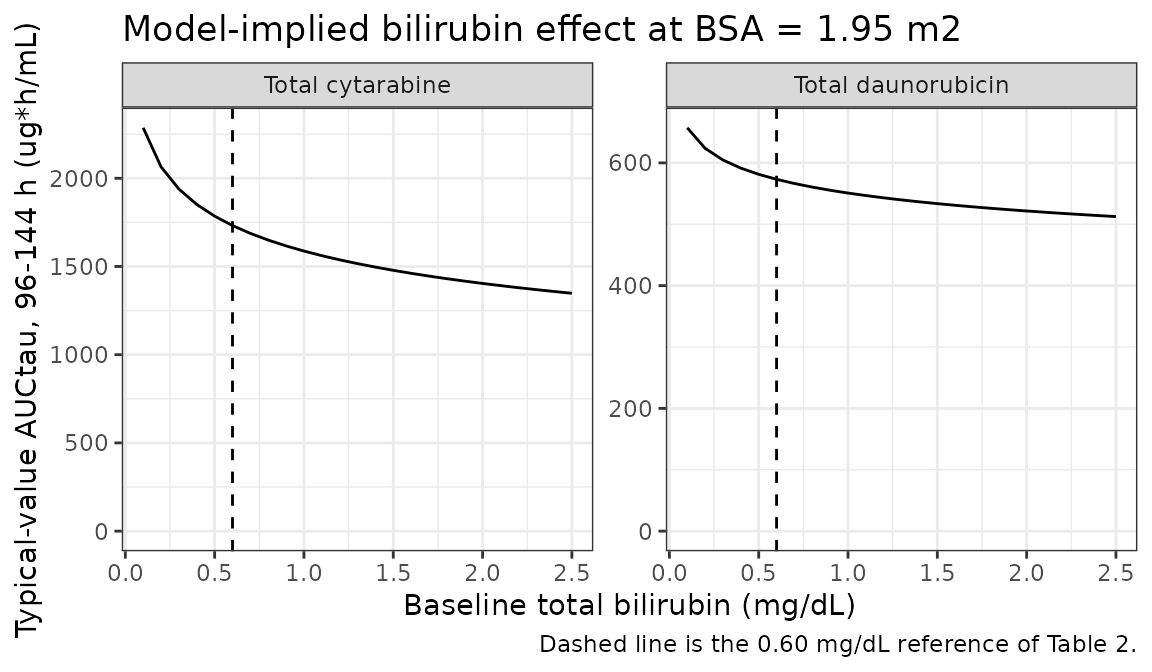

# All deterministic: typical values, no random effects, no cohort.
at_bili <- function(df, target) {
  df$auctau[which.min(abs(df$bili_mgdl - target))]
}

span <- do.call(rbind, lapply(split(bili_effect, bili_effect$analyte), function(d) {
  # The reference 0.60 mg/dL doubled to 1.20 mg/dL, which is also the boundary
  # between the two Table 3 bilirubin strata.
  a060 <- at_bili(d, 0.60)
  a120 <- at_bili(d, 1.20)
  tibble::tibble(
    analyte = d$analyte[1],
    pct_drop_full_range = 100 * (max(d$auctau) - min(d$auctau)) / max(d$auctau),
    pct_drop_per_doubling = 100 * (a060 - a120) / a060
  )
}))

# "The effect of bilirubin on CL was statistically significant, but the
# relationship was very shallow" (Results, both analytes). Quantified: a
# DOUBLING of bilirubin, which also crosses the Table 3 stratum boundary,
# must move typical exposure by less than 15%.
stopifnot(all(span$pct_drop_per_doubling < 15))
# The direction is itself a published claim -- "patients with higher bilirubin
# values were associated with a slightly faster CL" -- and is deterministic
# here because both exponents are positive and the solve carries no etas.
stopifnot(all(span$pct_drop_per_doubling > 0))
# Across the full 0.1-2.5 mg/dL range the fall is larger (the range spans a
# 25-fold change in bilirubin) but still bounded. A transcription slip of one
# decimal place in either exponent -- 1.97 instead of 0.197 -- would put this
# above 98%.
stopifnot(all(span$pct_drop_full_range < 60))

span |>
  dplyr::mutate(dplyr::across(dplyr::where(is.numeric), \(x) round(x, 1))) |>
  dplyr::rename(
    "Analyte" = analyte,
    "AUCtau decrease, 0.1 to 2.5 mg/dL (%)" = pct_drop_full_range,
    "AUCtau decrease per doubling, 0.60 to 1.20 mg/dL (%)" = pct_drop_per_doubling
  ) |>
  knitr::kable(caption = "Magnitude of the bilirubin effect over the observed range.")

Magnitude of the bilirubin effect over the observed range.
Analyte	AUCtau decrease, 0.1 to 2.5 mg/dL (%)	AUCtau decrease per doubling, 0.60 to 1.20 mg/dL (%)
Total cytarabine	41	11.2
Total daunorubicin	22	5.3

Frozen versus lyophilized formulation (daunorubicin only)

The frozen formulation, used throughout the phase 1 study 101, lowers all four daunorubicin disposition parameters. Because CL falls by 24% while Vc falls by only 20%, the net effect on exposure is an increase.

form_events <- function(frozen) {
  subj <- tibble::tibble(
    id = 1:2, BSA = 1.95, TBILI = 0.60 * 17.1,
    FORM_CPX351_FROZEN = frozen, bili_cat = "reference"
  )
  make_events(subj, mg_per_m2[["daunorubicin"]])
}

form_auc <- function(frozen) {
  sim <- rxode2::rxSolve(
    readModelDb("Wang_2019_daunorubicin_cpx351"),
    events = as.data.frame(form_events(frozen)), omega = NA
  ) |>
    as.data.frame() |>
    dplyr::filter(id == 1, time >= 96, time <= 144, !is.na(Cc)) |>
    dplyr::arrange(time)
  sum(diff(sim$time) * (head(sim$Cc, -1) + tail(sim$Cc, -1)) / 2)
}

auc_lyo <- form_auc(0)
#> Warning: multi-subject simulation without without 'omega'
auc_frz <- form_auc(1)
#> Warning: multi-subject simulation without without 'omega'

# Deterministic. exp(-0.275) = 0.760 on CL against exp(-0.221) = 0.802 on Vc,
# so the frozen arm must have the HIGHER AUCtau, by roughly 1/0.760 - 1 = 32%
# once distribution has equilibrated.
stopifnot(auc_frz > auc_lyo)

tibble::tibble(
  Formulation = c("Lyophilized (reference)", "Frozen"),
  `AUCtau, 96-144 h (ug*h/mL)` = signif(c(auc_lyo, auc_frz), 4),
  `Ratio to reference` = signif(c(1, auc_frz / auc_lyo), 3)
) |>
  knitr::kable(
    caption = "Typical-value daunorubicin exposure by CPX-351 formulation."
  )

Typical-value daunorubicin exposure by CPX-351 formulation.
Formulation	AUCtau, 96-144 h (ug*h/mL)	Ratio to reference
Lyophilized (reference)	573.2	1.00
Frozen	755.8	1.32

Assumptions and deviations

Covariate distributions are reconstructed, not observed. Body surface area and total bilirubin are drawn from log-normal distributions matched to the Table 1 medians, restricted to the Table 1 ranges, and for bilirubin calibrated so that 8.2% of the underlying distribution falls in the 1.2-3 mg/dL stratum as Table 1 reports. The two are drawn independently; any correlation between body size and hepatic function in the real cohort is not reproduced, which is the main reason the simulated stratum medians cannot be expected to match Table 3 exactly.
The two bilirubin strata are simulated at equal size (150 each) rather than in the 141:15 proportion of Table 3. Each arm still draws from the conditional distribution of the same fitted bilirubin lognormal on its own interval, so the quantity being compared is unchanged; only the precision of the upper stratum’s median improves. At the published 141:15 proportion that median moved by up to 32% between trial seeds, which would have forced a validation bound too loose to detect a real transcription error.
The published OMEGA blocks are encoded as diagonal. Results describe an OMEGA block on CL and Vc for cytarabine and on CL, Vc, Q and Vp for daunorubicin, but Tables S2 and S3 report only the diagonal variances. The off-diagonal covariances are not published anywhere on disk, so the etas are encoded as independent. This narrows the joint spread of derived quantities such as AUC relative to the authors’ model; the marginal variance of each parameter is unaffected.
No IIV on cytarabine Q and Vp. The Table 2 footnote states “BSV% for Q and Vp were not estimated due to high shrinkage on these parameters” and Table S2 carries no corresponding rows, so the final cytarabine model has three random effects (CL, Vc and the residual magnitude). No eta is invented for the other two parameters.
e_bsa_vc for cytarabine is 1.22, not the 1.21 printed in Table 2. Table S2 reports 1.22 with SE 0.186 and a 95% CI of 0.850-1.58, whose midpoint is 1.215; both printed figures are roundings of the same estimate. The supplement value is used because it carries the uncertainty that identifies it.
The bilirubin effect on daunorubicin clearance has a confidence interval spanning zero (0.0829, 95% CI -0.0198 to 0.186). It is retained because the paper built a full model with no reduction step, following Harrell, not because the effect is well identified.
Formulation is perfectly confounded with study. All 38 frozen-formulation patients came from study 101 and all 157 lyophilized patients from studies 206 and 301, so the fitted FORM_CPX351_FROZEN coefficients are a combined formulation-plus-study effect. The Discussion separately reports that “study phase had no measurable effect”, but that could not be assessed independently of formulation.
The exposure-response layer is not reproducible as a model and is not extracted. Wang 2019’s exposure-response analyses are Kaplan-Meier estimates, Cox proportional-hazards regressions and logistic regressions run in SAS. Table 4 reports adjusted hazard ratios and the text reports adjusted odds ratios, but no baseline hazard function and no logistic intercept are published, so neither a time-to-event nor a landmark probability model can be reconstructed from any on-disk source. The exposure variable itself, AUCtau from the population PK models, is reproduced above.
Renal function is not a covariate in either model, so the Table 3 renal stratification is discussed rather than simulated; see the covariate-effects section.
Molar masses are external constants. Cytarabine 243.22 g/mol and daunorubicin 527.52 g/mol are standard chemical values, used only in the descriptive molar-ratio figure and in no model parameter. The paper’s own statement that 1 mg cytarabine plus 0.44 mg daunorubicin constitutes a 5:1 molar ratio corroborates them.
The source reports two irreconcilable assay limits. The Bioanalytical Methods section gives a range of detection of 1000 to 100 000 ng/mL, while Results reports samples below a limit of quantification of 5 ng/mL. Nothing in the models depends on which is correct; the discrepancy is recorded in each model’s population$notes.