Ganitumab (Zhu 2013) • nlmixr2lib

Model and source

#> ℹ parameter labels from comments will be replaced by 'label()'

Citation: Zhu M, Gosselin NH, Kuchimanchi M, Johnson J, McCaffery I, Mouksassi MS, Loh E, Lu JF. Differential pharmacokinetics of ganitumab in patients with metastatic pancreatic cancer versus other advanced solid cancers. Clin Pharmacol Drug Dev. 2013;2(4):367-378. doi:10.1002/cpdd.48
Description: Two-compartment population PK model for intravenous ganitumab (AMG 479, anti-IGF1R IgG1 monoclonal antibody) in adults with metastatic pancreatic cancer or other advanced solid cancers, with pancreatic cancer type, body weight, serum albumin and serum creatinine on disposition (Zhu 2013)
Article: https://doi.org/10.1002/cpdd.48

Ganitumab (AMG 479) is a fully human IgG1 monoclonal antibody antagonist of the insulin-like growth factor-1 receptor (IGF1R). Zhu 2013 pooled three trials to build a two-compartment population PK model and found that pancreatic cancer type, not gemcitabine coadministration, was the dominant determinant of ganitumab disposition: typical clearance was 1.7-fold higher and typical central volume 1.3-fold higher in patients with metastatic pancreatic cancer than in patients with other advanced solid cancers.

Population

The estimation dataset comprised 99 patients contributing 1227 evaluable serum ganitumab concentrations from three trials (Zhu 2013 Supplemental Table 1):

Study	N with PK	Ganitumab dose	Cancer type	Regimen
Study 1 (NCT00630552)	35	12 mg/kg	Metastatic pancreatic cancer	Ganitumab + gemcitabine
Study 2 (NCT00562380)	53	1, 3, 10, 12 or 20 mg/kg	Advanced solid tumours	Ganitumab alone
Study 3 (NCT00974896)	11	6 or 12 mg/kg	Advanced solid tumours	Ganitumab + gemcitabine

All studies dosed intravenously once every 2 weeks. 62 of 99 patients (62.6%) had non-pancreatic cancer and 46 of 99 (46.5%) received concomitant gemcitabine. Two percent of samples were excluded as below the limit of quantification (LLOQ 20.2 ng/mL) or in error. Fitting used NONMEM VI level 1.1 with FOCE + INTERACTION.

A fourth trial (Study 4, NCT00626106; 104 patients with advanced breast cancer receiving 12 mg/kg plus hormonal therapy, 802 concentrations) was held out and used only for external qualification by visual predictive check; it is not part of the estimation dataset.

Zhu 2013 publishes no baseline-demographics table. The Results state only that “individual demographic data and disease characteristics for each study were normally distributed and were similar among studies”. Age, sex, race, and the medians and ranges of body weight, albumin and creatinine are therefore unavailable. This drives most of the Errata below, and it is why the virtual cohorts here vary random effects rather than covariates.

The same information is available programmatically via readModelDb("Zhu_2013_ganitumab")()$population.

Source trace

Per-parameter origin is recorded as an in-file comment beside each ini() entry in inst/modeldb/specificDrugs/Zhu_2013_ganitumab.R. Collected here for review:

Fixed-effect parameters as packaged.
Equation / parameter	Value	Source location
Two-compartment linear structure, CL / Q / Vc / Vp	n/a	Methods, “Base Model Development”; confirmed in Results, “Base PK Model Generation” (dMOF = -1255.55 vs 1-compartment)
IIV form `theta_i = theta_typ * exp(eta_i)`, diagonal OMEGA	n/a	Methods equation (1)
Residual error, proportional only	n/a	Methods equation (2) allows add + prop; Results, “Base PK Model Generation” states the final structure used “a proportional error model”; Table 1 reports no additive term
Continuous covariate form `(Cov/Cov_ref)^theta_eff`	n/a	Methods equation (3)
`lcl` = log(0.679)	0.679 L/day	Table 1, “Typical CL for non-pancreatic” (RSE 3.47%)
`lvc` = log(3.85)	3.85 L	Table 1, “Typical Vc for non-pancreatic cancer” (RSE 2.91%)
`lq` = log(0.626)	0.626 L/day	Table 1, “Q” (RSE 9.73%)
`lvp` = log(3.41)	3.41 L	Table 1, “Vp” (RSE 8.39%)
`e_wt_cl`	0.984	Table 1, “WT on CL” (RSE 12.8%)
`e_alb_cl`	-0.859	Table 1, “ALB on CL” (RSE 22.2%); sign from Results and Discussion prose, see Errata
`e_creat_cl`	-0.394	Table 1, “CR on CL” (RSE 24.7%); sign from Results and Discussion prose, see Errata
`e_wt_vc`	0.559	Table 1, “WT on Vc” (RSE 21.6%)
`e_panc_cl`	log(1.154 / 0.679)	Table 1, typical CL pancreatic 1.154 (RSE 5.84%) vs non-pancreatic 0.679 L/day
`e_panc_vc`	log(5.13 / 3.85)	Table 1, typical Vc pancreatic 5.13 (RSE 4.21%) vs non-pancreatic 3.85 L
`etalcl`	0.262^2	Table 1, “IIV CL 26.2%” (RSE 18.8%)
`etalvc`	0.217^2	Table 1, “IIV Vc 21.7%” (RSE 17.7%)
`etalq`	0.437^2	Table 1, “IIV Q 43.7%” (RSE 38.7%)
`etalvp`	0.602^2	Table 1, “IIV Vp 60.2%” (RSE 25.7%)
`propSd`	0.164	Table 1, “Proportional error 16.4%” (RSE 9.26%)
WT reference 74.7 kg	derived	Recovered by inverting the four published steady-state AUC values in Results; see “Recovering the reference body weight” below
ALB reference 40 g/L, CREAT reference 1 mg/dL	assumed	Not reported anywhere in Zhu 2013 or its supplement; see Errata

Parameter	Estimate	Label
lcl	-0.387134	Clearance in non-pancreatic cancer at reference covariates (L/day)
lvc	1.348070	Central volume of distribution in non-pancreatic cancer at reference covariates (L)
lq	-0.468405	Intercompartmental clearance (L/day)
lvp	1.226710	Peripheral volume of distribution (L)
e_wt_cl	0.984000	Power exponent of body weight on CL (unitless)
e_alb_cl	-0.859000	Power exponent of serum albumin on CL (unitless)
e_creat_cl	-0.394000	Power exponent of serum creatinine on CL (unitless)
e_wt_vc	0.559000	Power exponent of body weight on Vc (unitless)
e_panc_cl	0.530368	Exponential coefficient of pancreatic cancer type on CL (unitless)
e_panc_vc	0.287033	Exponential coefficient of pancreatic cancer type on Vc (unitless)
propSd	0.164000	Proportional residual error (fraction)

Reference covariate values

The model is centred on a non-pancreatic patient at the cohort median covariates, for whom every covariate term equals 1 and CL / Vc take their published typical values.

WT_REF    <- 74.7  # kg,    derived below
ALB_REF   <- 40    # g/L,   assumed (not published)
CREAT_REF <- 1     # mg/dL, assumed (not published)

Recovering the reference body weight

Zhu 2013 equation (3) defines the reference as “the median of the covariate among patients”, but the paper tabulates no medians. The parenthetical “(e.g., 70 kg for body weight)” in that same sentence illustrates what a reference value is; it is not a statement of the value used.

The reference weight is nevertheless identifiable from the paper’s own published exposures. At the median covariates every covariate term is 1, so AUCss = Dose / CL_typical, and with a mg/kg dose that inverts to WT_ref = AUCss * CL_typical / (mg/kg). Zhu 2013 Results reports four steady-state AUC values, which must all give the same answer:

auc_published <- tibble::tribble(
  ~arm,                      ~mgkg, ~auc_mg_day_mL, ~cl_typical,
  "Non-pancreatic 12 mg/kg",    12,           1.32,       0.679,
  "Non-pancreatic 20 mg/kg",    20,           2.20,       0.679,
  "Pancreatic 12 mg/kg",        12,           0.78,       1.154,
  "Pancreatic 20 mg/kg",        20,           1.29,       1.154
) |>
  mutate(wt_implied = auc_mg_day_mL * 1000 * cl_typical / mgkg)

auc_published |>
  dplyr::rename(
    "Arm"                        = arm,
    "Dose (mg/kg)"               = mgkg,
    "Published AUCss (mg*day/mL)" = auc_mg_day_mL,
    "Typical CL (L/day)"         = cl_typical,
    "Implied WT reference (kg)"  = wt_implied
  ) |>
  knitr::kable(digits = 2, caption = "Inverting the published steady-state AUC values for the reference weight.")

Inverting the published steady-state AUC values for the reference weight.
Arm	Dose (mg/kg)	Published AUCss (mg*day/mL)	Typical CL (L/day)	Implied WT reference (kg)
Non-pancreatic 12 mg/kg	12	1.32	0.68	74.69
Non-pancreatic 20 mg/kg	20	2.20	0.68	74.69
Pancreatic 12 mg/kg	12	0.78	1.15	75.01
Pancreatic 20 mg/kg	20	1.29	1.15	74.43

All four independently imply the same weight to three significant figures. The competing candidate, 70 kg, reproduces none of the four published AUC values:

candidate_check <- tidyr::expand_grid(
  wt_ref = c(70, 74.5, 74.7, 75.0),
  auc_published |> select(arm, mgkg, auc_mg_day_mL, cl_typical)
) |>
  mutate(auc_predicted = round(mgkg * wt_ref / cl_typical / 1000, 2)) |>
  group_by(wt_ref) |>
  summarise(
    n_matching = sum(auc_predicted == auc_mg_day_mL),
    predicted  = paste(sprintf("%.2f", auc_predicted), collapse = ", "),
    .groups    = "drop"
  )

candidate_check |>
  dplyr::rename(
    "Candidate WT reference (kg)"          = wt_ref,
    "Published AUCss reproduced (out of 4)" = n_matching,
    "Predicted AUCss (mg*day/mL)"          = predicted
  ) |>
  knitr::kable(caption = "Only 74.7 kg reproduces all four published steady-state AUC values.")

Only 74.7 kg reproduces all four published steady-state AUC values.
Candidate WT reference (kg)	Published AUCss reproduced (out of 4)	Predicted AUCss (mg*day/mL)
70.0	0	1.24, 2.06, 0.73, 1.21
74.5	2	1.32, 2.19, 0.77, 1.29
74.7	4	1.32, 2.20, 0.78, 1.29
75.0	1	1.33, 2.21, 0.78, 1.30


stopifnot(
  # Exactly one candidate reproduces all four; 70 kg reproduces none.
  candidate_check$n_matching[candidate_check$wt_ref == WT_REF] == 4L,
  candidate_check$n_matching[candidate_check$wt_ref == 70]     == 0L,
  sum(candidate_check$n_matching == 4L) == 1L,
  # And the packaged constant agrees with the mean of the four inversions.
  abs(mean(auc_published$wt_implied) - WT_REF) < 0.1
)

Albumin and creatinine admit no equivalent inversion: no published quantity depends on them separately, so their reference values are assumed. See Errata.

Virtual cohort

Original observed data are not publicly available, and Zhu 2013 publishes no demographic distributions, so a covariate-varying virtual population would be fabrication rather than replication. The cohorts below therefore hold covariates at the reference values and vary only the model’s own random effects, which are published. Covariate effects are exercised separately, deterministically, in the sensitivity section.

INFUSION_DUR <- 1 / 24  # days; see Errata -- Zhu 2013 does not state the duration
II           <- 14      # days between doses (Q2W, Supplemental Table 1 footnote a)

arms <- tibble::tribble(
  ~arm,                      ~TUMTP_PANC, ~mgkg,
  "Non-pancreatic 12 mg/kg",          0L,    12,
  "Non-pancreatic 20 mg/kg",          0L,    20,
  "Pancreatic 12 mg/kg",              1L,    12,
  "Pancreatic 20 mg/kg",              1L,    20
)

# Build one arm as a self-contained event table. `id_offset` keeps subject IDs
# disjoint across arms; duplicate IDs are silently merged by rxSolve.
make_arm <- function(arm_row, n, n_doses, obs_times, id_offset = 0L) {
  ids <- id_offset + seq_len(n)
  amt <- arm_row$mgkg * WT_REF
  doses <- tidyr::expand_grid(id = ids, time = II * (seq_len(n_doses) - 1L)) |>
    mutate(amt = amt, evid = 1L, cmt = "central", dur = INFUSION_DUR)
  obs <- tidyr::expand_grid(id = ids, time = obs_times) |>
    mutate(amt = NA_real_, evid = 0L, cmt = "central", dur = NA_real_)
  bind_rows(doses, obs) |>
    mutate(
      WT = WT_REF, ALB = ALB_REF, CREAT = CREAT_REF,
      TUMTP_PANC = arm_row$TUMTP_PANC,
      arm = arm_row$arm, mgkg = arm_row$mgkg
    ) |>
    arrange(id, time, desc(evid))
}

Simulation

Typical-value steady state

Twenty Q2W doses take every arm well past steady state (Zhu 2013 predicts steady state in 7 weeks for non-pancreatic and 5 weeks for pancreatic cancer). The final dosing interval is sampled finely so trapezoidal AUC resolves the post-infusion peak.

n_doses  <- 20L
t_last   <- II * (n_doses - 1L)
grid_tau <- sort(unique(c(
  seq(0, 0.5, by = 0.005), seq(0.5, 2, by = 0.05), seq(2, II, by = 0.2), II
)))

events_ss <- bind_rows(lapply(seq_len(nrow(arms)), function(i) {
  make_arm(arms[i, ], n = 1L, n_doses = n_doses,
           obs_times = t_last + grid_tau, id_offset = i - 1L)
}))
stopifnot(!anyDuplicated(unique(events_ss[, c("id", "time", "evid")])))

mod         <- readModelDb("Zhu_2013_ganitumab")
mod_typical <- rxode2::zeroRe(mod)
#> ℹ parameter labels from comments will be replaced by 'label()'
sim_ss <- rxode2::rxSolve(mod_typical, events = events_ss,
                          keep = c("arm", "mgkg", "TUMTP_PANC")) |>
  as.data.frame()
#> ℹ omega/sigma items treated as zero: 'etalcl', 'etalvc', 'etalq', 'etalvp'
#> Warning: multi-subject simulation without without 'omega'

Typical disposition parameters

typ <- sim_ss |>
  group_by(arm) |>
  summarise(cl = first(cl), vc = first(vc), q = first(q), vp = first(vp),
            .groups = "drop") |>
  mutate(vss = vc + vp)

typ |>
  dplyr::rename(
    "Arm"           = arm,
    "CL (L/day)"    = cl,
    "Vc (L)"        = vc,
    "Q (L/day)"     = q,
    "Vp (L)"        = vp,
    "Vc + Vp (L)"   = vss
  ) |>
  knitr::kable(digits = 3, caption = "Typical disposition parameters at the reference covariates.")

Typical disposition parameters at the reference covariates.
Arm	CL (L/day)	Vc (L)	Q (L/day)	Vp (L)	Vc + Vp (L)
Non-pancreatic 12 mg/kg	0.679	3.85	0.626	3.41	7.26
Non-pancreatic 20 mg/kg	0.679	3.85	0.626	3.41	7.26
Pancreatic 12 mg/kg	1.154	5.13	0.626	3.41	8.54
Pancreatic 20 mg/kg	1.154	5.13	0.626	3.41	8.54


np <- typ |> filter(arm == "Non-pancreatic 12 mg/kg")
pc <- typ |> filter(arm == "Pancreatic 12 mg/kg")

stopifnot(
  # Table 1 typical values, reproduced exactly by construction.
  abs(np$cl - 0.679) < 1e-9, abs(np$vc - 3.85) < 1e-9,
  abs(pc$cl - 1.154) < 1e-9, abs(pc$vc - 5.13) < 1e-9,
  abs(np$q  - 0.626) < 1e-9, abs(np$vp - 3.41) < 1e-9,
  # Discussion: "the typical ganitumab Vc + Vp in patients with non-pancreatic
  # cancer was 7.3 L", and "higher Vc + Vp was found in patients with
  # pancreatic cancer (8.5 L)". These are INDEPENDENT of the typical-value
  # round trip above -- they test that Vp is not double-counted per arm.
  round(np$vc + np$vp, 1) == 7.3,
  round(pc$vc + pc$vp, 1) == 8.5,
  # Abstract and Results: CL 1.7-fold and Vc 1.3-fold higher in pancreatic.
  round(pc$cl / np$cl, 1) == 1.7,
  round(pc$vc / np$vc, 1) == 1.3
)

Terminal half-life

Zhu 2013 reports a “calculated median elimination half-life” of approximately 10 days in non-pancreatic and approximately 7 days in pancreatic cancer. The fit below regresses log(Cc) well after a single dose, where the distribution phase has decayed, and is cross-checked against the closed-form two-compartment beta eigenvalue.

events_wash <- bind_rows(lapply(seq_len(nrow(arms)), function(i) {
  make_arm(arms[i, ], n = 1L, n_doses = 1L,
           obs_times = seq(60, 140, by = 1), id_offset = i - 1L)
}))
sim_wash <- rxode2::rxSolve(mod_typical, events = events_wash, keep = "arm") |>
  as.data.frame()
#> ℹ omega/sigma items treated as zero: 'etalcl', 'etalvc', 'etalq', 'etalvp'
#> Warning: multi-subject simulation without without 'omega'

thalf <- sim_wash |>
  group_by(arm) |>
  summarise(
    t_half_fitted = log(2) / -stats::coef(stats::lm(log(Cc) ~ time))[["time"]],
    cl = first(cl), vc = first(vc), q = first(q), vp = first(vp),
    .groups = "drop"
  ) |>
  mutate(
    k10 = cl / vc, k12 = q / vc, k21 = q / vp,
    s   = k10 + k12 + k21,
    beta = (s - sqrt(s^2 - 4 * k10 * k21)) / 2,
    t_half_closed_form = log(2) / beta,
    published = ifelse(grepl("^Pancreatic", arm), 7, 10)
  )

thalf |>
  select(arm, t_half_fitted, t_half_closed_form, published) |>
  dplyr::rename(
    "Arm"                          = arm,
    "Fitted terminal t1/2 (days)"  = t_half_fitted,
    "Closed-form t1/2 (days)"      = t_half_closed_form,
    "Zhu 2013 reported (days)"     = published
  ) |>
  knitr::kable(digits = 2, caption = "Terminal half-life vs the reported approximate values.")

Terminal half-life vs the reported approximate values.
Arm	Fitted terminal t1/2 (days)	Closed-form t1/2 (days)	Zhu 2013 reported (days)
Non-pancreatic 12 mg/kg	9.65	9.65	10
Non-pancreatic 20 mg/kg	9.65	9.65	10
Pancreatic 12 mg/kg	7.31	7.31	7
Pancreatic 20 mg/kg	7.31	7.31	7


stopifnot(
  # The washout fit must recover the analytic eigenvalue, not merely be close
  # to the paper's rounded figure.
  all(abs(thalf$t_half_fitted - thalf$t_half_closed_form) /
        thalf$t_half_closed_form < 0.01),
  # Zhu 2013 reports these only to the nearest day ("approximately"), so the
  # test is that each rounds to the published integer.
  all(round(thalf$t_half_closed_form) == thalf$published)
)

PKNCA validation

NCA is run over the final dosing interval, which contains exactly one dose and one full Q2W interval, giving AUCtau at steady state.

conc_ss <- sim_ss |>
  dplyr::filter(!is.na(Cc)) |>
  dplyr::select(id, time, Cc, arm)

dose_ss <- events_ss |>
  dplyr::filter(evid == 1L, time == t_last) |>
  dplyr::select(id, time, amt, arm)

conc_obj <- PKNCA::PKNCAconc(conc_ss, Cc ~ time | arm + id)
dose_obj <- PKNCA::PKNCAdose(dose_ss, amt ~ time | arm + id)

intervals <- data.frame(
  start = t_last, end = t_last + II,
  cmax = TRUE, tmax = TRUE, cmin = TRUE, auclast = TRUE
)

nca_res <- PKNCA::pk.nca(PKNCA::PKNCAdata(conc_obj, dose_obj, intervals = intervals))

Comparison against published NCA

Zhu 2013 Results reports steady-state AUC in mgday/mL; the model works in ug/mL and days, so the published values are multiplied by 1000 to give ugday/mL. Note that AUCtau,ss = Dose / CL exactly, so this comparison is independent of the assumed infusion duration.

published_nca <- auc_published |>
  transmute(arm, auclast = auc_mg_day_mL * 1000)

cmp <- nlmixr2lib::ncaComparisonTable(
  simulated     = nca_res,
  reference     = published_nca,
  by            = "arm",
  params        = "auclast",
  units         = c(auclast = "ug*day/mL"),
  tolerance_pct = 20
)

knitr::kable(
  cmp,
  caption = "Simulated steady-state AUCtau vs Zhu 2013 Results. * differs from reference by >20%.",
  align   = c("l", "l", "r", "r", "r")
)

Simulated steady-state AUCtau vs Zhu 2013 Results. * differs from reference by >20%.
NCA parameter	arm	Reference	Simulated	% diff
AUClast (ug*day/mL)	Non-pancreatic 12 mg/kg	1320	1320	+0.0%
AUClast (ug*day/mL)	Non-pancreatic 20 mg/kg	2200	2200	+0.0%
AUClast (ug*day/mL)	Pancreatic 12 mg/kg	780	777	-0.4%
AUClast (ug*day/mL)	Pancreatic 20 mg/kg	1290	1290	+0.4%


nca_wide <- as.data.frame(nca_res) |>
  select(arm, PPTESTCD, PPORRES) |>
  tidyr::pivot_wider(names_from = PPTESTCD, values_from = PPORRES) |>
  left_join(published_nca, by = "arm", suffix = c("", "_published")) |>
  left_join(typ |> select(arm, cl), by = "arm") |>
  left_join(arms |> select(arm, mgkg), by = "arm") |>
  mutate(
    dose_mg        = mgkg * WT_REF,
    auc_dose_by_cl = dose_mg / cl,
    pct_vs_published = 100 * (auclast - auclast_published) / auclast_published,
    pct_vs_identity  = 100 * (auclast - auc_dose_by_cl) / auc_dose_by_cl
  )

stopifnot(
  # (a) Numerical: trapezoidal AUCtau must reproduce the closed form Dose/CL.
  #     Both sides use the same drawn parameters, so this is pure quadrature
  #     error and a tight bound is the right test.
  all(abs(nca_wide$pct_vs_identity) < 0.1),
  # (b) Structural: AUCtau must reproduce all four published values. The
  #     residual is the paper's own 2-decimal rounding (<= 0.5%).
  all(abs(nca_wide$pct_vs_published) < 1),
  # Guard: the comparison actually had all four arms to test.
  nrow(nca_wide) == 4L, !anyNA(nca_wide$pct_vs_published)
)

The pancreatic-versus-non-pancreatic exposure gap that motivates the paper’s dosing conclusion falls straight out:

gap <- nca_wide |>
  select(arm, mgkg, auclast) |>
  mutate(group = ifelse(grepl("^Pancreatic", arm), "pancreatic", "non_pancreatic")) |>
  select(mgkg, group, auclast) |>
  tidyr::pivot_wider(names_from = group, values_from = auclast) |>
  mutate(ratio = non_pancreatic / pancreatic)

gap |>
  dplyr::rename(
    "Dose (mg/kg)"                    = mgkg,
    "Non-pancreatic AUCss (ug*day/mL)" = non_pancreatic,
    "Pancreatic AUCss (ug*day/mL)"     = pancreatic,
    "Exposure ratio"                   = ratio
  ) |>
  knitr::kable(digits = c(0, 0, 0, 2), caption = "Steady-state exposure gap by cancer type.")

Steady-state exposure gap by cancer type.
Dose (mg/kg)	Non-pancreatic AUCss (ug*day/mL)	Pancreatic AUCss (ug*day/mL)	Exposure ratio
12	1320	777	1.7
20	2200	1295	1.7


stopifnot(
  # The exposure ratio is the reciprocal of the 1.7-fold CL difference.
  all(abs(gap$ratio - 1.154 / 0.679) < 0.02)
)

Replicate published figures

Figure 1 analogue – projected profiles over the first four doses

Zhu 2013 Figure 1 overlays observed breast-cancer concentrations (Study 4, 12 mg/kg Q2W) on the median and 90% prediction interval projected from the final model for the first four doses. Breast cancer is a non-pancreatic type, so TUMTP_PANC = 0. The observed data are not available, so only the projection is reproduced; the pancreatic arm is added for contrast.

# rxode2 draws etas from its own RNG, which base `set.seed()` does not reach;
# `rxSetSeed()` is what makes the cohort below reproducible.
rxode2::rxSetSeed(20130926)
set.seed(20130926)
n_per_arm <- 200L
grid_vpc  <- sort(unique(c(
  seq(0, 56, by = 0.5),
  as.vector(outer(II * (0:3), c(0.04, 0.1, 0.25, 0.5, 1), "+"))
)))
grid_vpc <- grid_vpc[grid_vpc <= 56]

vpc_arms <- arms |> filter(mgkg == 12)

# One rxSolve per arm rather than one pooled call, for two reasons. (1) Cost:
# rxSolve on an rxUi scales super-linearly in subjects per call, so two calls of
# 200 are markedly cheaper than one of 400. (2) Reseeding inside the loop gives
# the two arms COMMON RANDOM NUMBERS -- subject i draws the same etas in both
# arms, so the pancreatic-vs-non-pancreatic contrast below is paired and
# reflects only the cancer-type effect, not sampling noise between two
# independent cohorts.
sim_vpc <- bind_rows(lapply(seq_len(nrow(vpc_arms)), function(i) {
  rxode2::rxSetSeed(20130926)
  ev <- make_arm(vpc_arms[i, ], n = n_per_arm, n_doses = 4L,
                 obs_times = grid_vpc, id_offset = 0L)
  stopifnot(!anyDuplicated(unique(ev[, c("id", "time", "evid")])))
  rxode2::rxSolve(mod, events = ev, keep = c("arm", "TUMTP_PANC")) |>
    as.data.frame()
}))
#> ℹ parameter labels from comments will be replaced by 'label()'

vpc_band <- sim_vpc |>
  # Drop t = 0: the first infusion has not yet delivered any drug there, so Cc
  # is exactly 0 and would be dropped by the log scale anyway.
  filter(!is.na(Cc), time > 0) |>
  group_by(arm, time) |>
  summarise(
    Q05 = quantile(Cc, 0.05), Q50 = median(Cc), Q95 = quantile(Cc, 0.95),
    .groups = "drop"
  )

ggplot(vpc_band, aes(time, Q50)) +
  geom_ribbon(aes(ymin = Q05, ymax = Q95), alpha = 0.25) +
  geom_line(linewidth = 0.7) +
  facet_wrap(~arm) +
  scale_y_log10() +
  labs(
    x = "Time (days)", y = "Ganitumab serum concentration (ug/mL)",
    title = "Projected ganitumab profiles, 12 mg/kg Q2W, first four doses",
    caption = "Replicates the projection in Figure 1 of Zhu 2013."
  ) +
  theme_bw()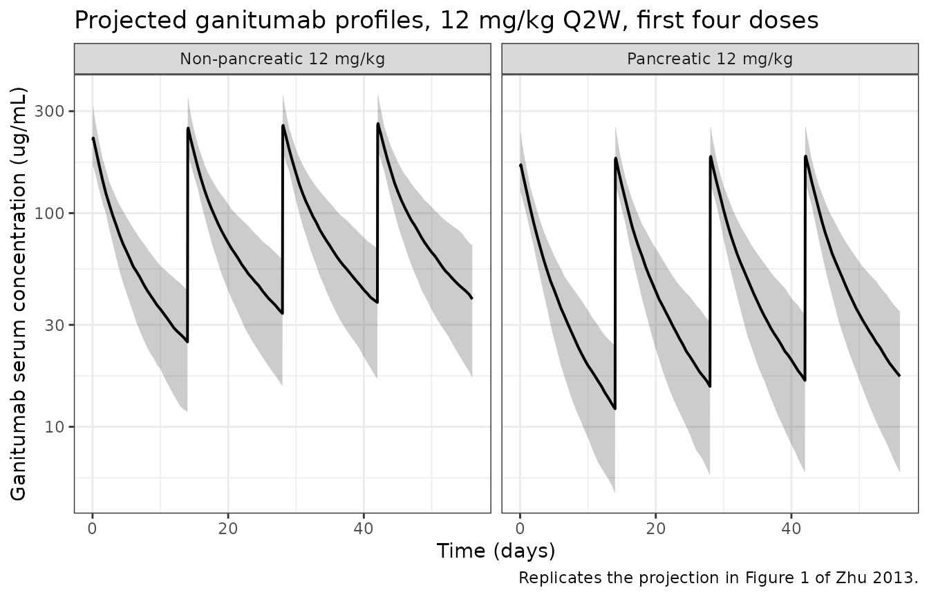

Replicates the projection in Figure 1 of Zhu 2013 (median and 90% prediction interval, 12 mg/kg Q2W, first four doses), with the pancreatic-cancer arm added for contrast.


stopifnot(
  # Guard: the band was actually computed over both arms and the full window.
  nrow(vpc_band) > 0L, dplyr::n_distinct(vpc_band$arm) == 2L,
  # Every simulated concentration from the end of the first infusion onward is
  # above the assay LLOQ of 20.2 ng/mL (0.0202 ug/mL), consistent with the
  # paper excluding only 2% of samples as below quantification or in error.
  min(vpc_band$Q05[vpc_band$time >= 1]) > 0.0202,
  # Cancer-type separation, asserted PER SUBJECT rather than on cohort
  # quantiles. The two arms share eta draws (common random numbers), so subject
  # i differs between arms only by TUMTP_PANC -- every one of the 200 subjects
  # must therefore show a lower trough in the pancreatic arm. This is an exact
  # 200/200 test rather than a noise-limited comparison of two distributions.
  {
    tail_paired <- sim_vpc |>
      filter(!is.na(Cc), time == max(grid_vpc)) |>
      select(id, arm, Cc) |>
      mutate(arm = ifelse(grepl("^Pancreatic", arm), "panc", "nonpanc")) |>
      tidyr::pivot_wider(names_from = arm, values_from = Cc)
    nrow(tail_paired) == n_per_arm && all(tail_paired$panc < tail_paired$nonpanc)
  }
)

Covariate sensitivity

The published exponents are the transferable part of the covariate model. This panel sweeps each continuous covariate deterministically (random effects zeroed, all other covariates at reference) and reports the resulting steady-state exposure relative to the reference patient. AUCss is inversely proportional to CL, so each curve is (Cov / Cov_ref)^(-exponent).

cov_grid <- bind_rows(
  tibble(covariate = "WT (kg)",    value = seq(45, 115, by = 5)) |>
    mutate(WT = value, ALB = ALB_REF, CREAT = CREAT_REF),
  tibble(covariate = "ALB (g/L)",  value = seq(25, 50, by = 2.5)) |>
    mutate(WT = WT_REF, ALB = value, CREAT = CREAT_REF),
  tibble(covariate = "CREAT (mg/dL)", value = seq(0.5, 1.6, by = 0.1)) |>
    mutate(WT = WT_REF, ALB = ALB_REF, CREAT = value)
) |>
  mutate(id = row_number(), TUMTP_PANC = 0L)

events_cov <- bind_rows(
  cov_grid |> mutate(time = 0, amt = 12 * WT_REF, evid = 1L, cmt = "central",
                     dur = INFUSION_DUR),
  cov_grid |> mutate(time = 1, amt = NA_real_, evid = 0L, cmt = "central",
                     dur = NA_real_)
) |>
  arrange(id, time, desc(evid))

# Each row of `cov_grid` is its own subject, so the covariate labels are
# recovered by joining on `id` rather than via `keep=`. rxSolve does not return
# a column named `value`, so keeping it is not an option here.
sim_cov <- rxode2::rxSolve(mod_typical, events = events_cov) |>
  as.data.frame() |>
  mutate(id = as.integer(as.character(id))) |>
  group_by(id) |>
  summarise(cl = first(cl), .groups = "drop") |>
  left_join(cov_grid |> select(id, covariate, value), by = "id") |>
  mutate(auc_relative = 0.679 / cl)
#> ℹ omega/sigma items treated as zero: 'etalcl', 'etalvc', 'etalq', 'etalvp'
#> Warning: multi-subject simulation without without 'omega'

stopifnot(
  # Guard: the join must cover every grid point, or a silently-dropped covariate
  # arm would make the slope tests below vacuous.
  nrow(sim_cov) == nrow(cov_grid), !anyNA(sim_cov$covariate), !anyNA(sim_cov$cl)
)

ggplot(sim_cov, aes(value, auc_relative)) +
  geom_line() +
  geom_hline(yintercept = 1, linetype = "dashed", colour = "grey40") +
  facet_wrap(~covariate, scales = "free_x") +
  labs(x = "Covariate value", y = "Steady-state exposure relative to reference") +
  theme_bw()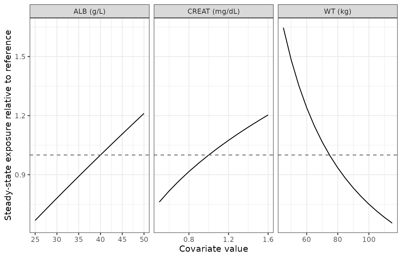

Deterministic covariate sensitivity of steady-state exposure, non-pancreatic patient at 12 mg/kg Q2W.


stopifnot(
  # Each curve passes through 1 at its own reference value.
  abs(sim_cov$auc_relative[sim_cov$covariate == "ALB (g/L)" &
                             sim_cov$value == ALB_REF] - 1) < 1e-8,
  abs(sim_cov$auc_relative[sim_cov$covariate == "CREAT (mg/dL)" &
                             sim_cov$value == CREAT_REF] - 1) < 1e-8,
  # Directions match the published signs: exposure falls with weight, and
  # rises with albumin and with creatinine.
  {
    slope <- function(cv) {
      d <- sim_cov |> filter(covariate == cv) |> arrange(value)
      stats::coef(stats::lm(log(auc_relative) ~ log(value), data = d))[["log(value)"]]
    }
    all(abs(slope("WT (kg)")       - (-0.984)) < 1e-6,
        abs(slope("ALB (g/L)")     - ( 0.859)) < 1e-6,
        abs(slope("CREAT (mg/dL)") - ( 0.394)) < 1e-6)
  }
)

Cross-check against the paper’s non-compartmental clearances

Zhu 2013 also reports mean (SD) NCA clearances in mL/kg/day from individual intensive profiles. These are shown for completeness but are not asserted on: they are arithmetic means over small single-cycle subsets whose covariate values are unpublished, obtained from sampling windows of 336-672 h against a terminal half-life of 7-10 days.

nca_cl <- tibble::tribble(
  ~cohort,                              ~n,  ~mean_ml_kg_day, ~sd, ~panc,
  "Non-pancreatic, no gemcitabine (Study 2)", 33L, 10.1, 3.8, 0L,
  "Non-pancreatic, + gemcitabine (Study 3)",  11L, 11.1, 3.1, 0L,
  "Pancreatic, + gemcitabine (Study 1)",      13L, 21.1, 6.4, 1L
) |>
  mutate(
    model_ml_kg_day = ifelse(panc == 1L, 1.154, 0.679) / WT_REF * 1000,
    pct_diff        = 100 * (model_ml_kg_day - mean_ml_kg_day) / mean_ml_kg_day
  )

nca_cl |>
  select(cohort, n, mean_ml_kg_day, sd, model_ml_kg_day, pct_diff) |>
  dplyr::rename(
    "Cohort"                          = cohort,
    "N"                               = n,
    "Zhu 2013 NCA mean CL (mL/kg/day)" = mean_ml_kg_day,
    "SD"                              = sd,
    "Model typical CL (mL/kg/day)"     = model_ml_kg_day,
    "% difference"                     = pct_diff
  ) |>
  knitr::kable(digits = 1, caption = "Model typical CL vs the paper's non-compartmental clearances (context only, not asserted).")

Model typical CL vs the paper’s non-compartmental clearances (context only, not asserted).
Cohort	N	Zhu 2013 NCA mean CL (mL/kg/day)	SD	Model typical CL (mL/kg/day)	% difference
Non-pancreatic, no gemcitabine (Study 2)	33	10.1	3.8	9.1	-10.0
Non-pancreatic, + gemcitabine (Study 3)	11	11.1	3.1	9.1	-18.1
Pancreatic, + gemcitabine (Study 1)	13	21.1	6.4	15.4	-26.8

The model’s typical CL sits within one SD of the two non-pancreatic NCA means but is 27% below the pancreatic NCA mean. That direction is expected: NCA Dose / AUCinf overestimates CL whenever the terminal phase is under-sampled, and Study 1’s pancreatic cohort was sampled to 336 h against a ~7-day terminal half-life. The population estimate, which borrows the terminal phase across all 99 subjects, is the more reliable of the two. The model was not adjusted to close this gap.

Assumptions and deviations

Errata and unresolved items in the source

Negative signs on the albumin and creatinine exponents. Most text and markdown extractions of this Wiley PDF render “ALB on CL” and “CR on CL” as bare magnitudes, which invites reading them as positive. They are negative. The journal encodes the minus sign as the C0 control byte 0x03 rather than an ASCII hyphen, so decoding the byte stream recovers the signs directly – pdftotext -layout | cat -A over Table 1 gives:
```
WT on CL       0.984 (12.8)     <- no control byte: POSITIVE
ALB on CL    ^C0.859 (22.2)     <- ^C = 0x03 = minus: NEGATIVE
CR on CL     ^C0.394 (24.7)     <- ^C = 0x03 = minus: NEGATIVE
```
The within-table contrast is what makes this conclusive rather than suggestive: weight carries no control byte while albumin and creatinine both do, so the absent signs are not a blanket artifact applied uniformly to every row. The same encoding shows up in the Results prose, where the dMOF values appear as ^C1255.55, ^C55.971 and ^C34.848 – all quantities that must be negative. Corroborated independently by the paper’s prose in three places: Results (“higher baseline albumin and creatinine values were associated with decreased ganitumab CL”), and Discussion (“baseline albumin was negatively correlated with CL for all cancer types” and “lower muscle mass in patients with pancreatic cancer may lead to lower creatinine levels and higher CL of ganitumab”). Encoded as -0.859 and -0.394.
Reference body weight 74.7 kg, not the 70 kg named in the Methods. Zhu 2013 equation (3) defines the reference as the cohort median but reports no medians; the “(e.g., 70 kg for body weight)” parenthetical in that sentence illustrates the concept rather than stating the value. The reference weight was recovered by inverting the four published steady-state AUC values, which agree on 74.7 kg to three significant figures and rule out 70 kg outright (see “Recovering the reference body weight”). This is a derived, non-paper-stated value.
Reference albumin (40 g/L) and creatinine (1 mg/dL) are assumed. These are rounded standard adult values. Zhu 2013 reports no baseline-demographics table, and no published quantity depends on albumin or creatinine separately, so no inversion analogous to the weight derivation is possible. The published exponents are unaffected and are the transferable part of the covariate model; a user applying this model to their own cohort should re-centre on their own medians, which rescales the typical CL but preserves every covariate effect. Zhu 2013’s Discussion notes that cachexia lowers creatinine in pancreatic cancer, so the true cohort median may sit below 1 mg/dL.
Infusion duration is not stated anywhere in Zhu 2013 or its supplement. The vignette uses a 1-hour intravenous infusion, consistent with the Supplemental Table 1 sampling schemes (“prior and end of infusion”; cycle-1 samples at 0, 1 and 3 h). The choice affects Cmax and Tmax only: AUCtau,ss = Dose / CL is exactly independent of it, so every AUC assertion in this vignette is immune to the assumption. The model file itself carries no infusion duration – it is supplied by the event table.
No demographic distributions are published, so the virtual cohorts vary only the model’s published random effects and hold covariates at the reference values. A covariate-varying virtual population would be invention rather than replication. Covariate effects are instead demonstrated deterministically.
IIV scale. Zhu 2013 Table 1 reports each IIV as a percentage. Under the paper’s own notation in equation (1) – “estimated variance v^2 (hereafter … v is referred to as OMEGA)” – the tabulated percentage is OMEGA, the SD on the log scale, so the variance is (percent / 100)^2. This reading is corroborated by the residual error: Table 1’s “Proportional error (%) 16.4” matches the Results text “RV decreased from 31.5% to 16.5%”, which is an SD-scale percentage rather than a variance. The alternative back-transform omega^2 = log(1 + CV^2) would change the IIV on Vp (60.2%) by about 8% and the others by under 2%.
Residual error is proportional only. Methods equation (2) writes a combined additive-plus-proportional model, but the final structure is proportional: the Results state the base model used “a proportional error model”, and Table 1 reports no additive term.
Inter-occasion variability was evaluated and not included (“Since CL and Vc were similar across occasions, and changes in either parameter over time were negligible, IOV was not incorporated in the base model”), so the model carries none.

Covariates screened but not retained

Zhu 2013 screened a wide covariate set and retained only weight, albumin, creatinine and cancer type. The screening ran in two stages, and the model file records which stage rejected each covariate:

Stage 1 (Methods) – graphical exploration plus Pearson correlation against posthoc CL and Vc. Twenty-three items entered: age, WT, BMI, sex, race, CR, ALB, total bilirubin, AST, ALT, ALP, disease stage at enrollment, ECOG performance status, platelet count, neutrophils, fasting blood glucose, BUN, LDH, IGF-1, IGFBP3, gemcitabine coadministration, study, and MDRD-estimated GFR. Creatinine clearance derived from WT and CR was deliberately never screened, as collinear with its own inputs.
Stage 2 (Results) – formal stepwise forward addition at P < .01 followed by backward elimination at P < .005, applied to the stage-1 survivors: on CL, WT, sex, CR, ALB, AST, ALT, ALP, platelets, neutrophils, IGF-1, IGFBP3, ECOG, gemcitabine and GFR; on Vc, WT, sex, ALP and gemcitabine.

The rejected covariates are documented in the model file’s covariatesDataExcluded metadata rather than covariateData, since none carries a published point estimate:

Covariates screened by Zhu 2013 but not retained in the final model.
Covariate	Description
CONMED_GEMCITABINE	Concomitant gemcitabine coadministration
AGE	Age
SEXF	Sex
BMI	Body mass index
TBILI	Total bilirubin
AST	Aspartate aminotransferase
ALT	Alanine aminotransferase
ALP	Alkaline phosphatase
LDH	Lactate dehydrogenase
BUN	Blood urea nitrogen
NEUT	Absolute neutrophil count
ECOG_GE1	ECOG performance status at or above 1
CRCL	MDRD-estimated glomerular filtration rate
FPG	Fasting blood glucose

Six screened concepts are recorded as a comment in the model file rather than as covariatesDataExcluded entries, because no entry can be written honestly for them. Platelet count, IGF-1, IGFBP3 and disease stage have no canonical covariate-register name, and registering one for a covariate that no model references would leave an unused name in the register. Race is registered only as per-group indicators (RACE_WHITE, RACE_BLACK, …), and Zhu 2013 never states which race levels its cohort contained, so no indicator can be named without inventing the composition. Study was screened as a categorical, but the paper pools Studies 1-3 and reports no per-study coefficient.

One elimination is worth singling out. MDRD-estimated GFR reached stage 2 on CL and was dropped, while serum creatinine – the input to that very estimate – was retained. That is not a contradiction but a clue to the mechanism: a 150 kDa IgG1 is not renally cleared, so creatinine is not acting here as a renal-function marker. It is acting as a marker of muscle mass, which is exactly the reading the Discussion gives when it attributes the faster pancreatic clearance to cachexia – “lower muscle mass in patients with pancreatic cancer may lead to lower creatinine levels and higher CL of ganitumab”. Normalising creatinine into a GFR estimate divides out the very signal that made it predictive.

The most consequential of these is gemcitabine coadministration. Tested alone it was significant (dMOF = -34.848, P < .001), but it was confounded with pancreatic cancer type, which was the stronger effect (dMOF = -55.971); once cancer type entered the model gemcitabine became non-significant (P > .2). The paper corroborated this non-compartmentally, and the resulting conclusion – that disease state rather than the chemotherapy backbone drives ganitumab exposure – is the paper’s headline finding.