Micafungin (Martial 2017)
Source:vignettes/articles/Martial_2017_micafungin.Rmd
Martial_2017_micafungin.RmdModel and source
- Citation: Martial LC, ter Heine R, Schouten JA, Hunfeld NG, van Leeuwen HJ, Verweij PE, de Lange DW, Pickkers P, Bruggemann RJ; FANTASTIC Consortium. Population Pharmacokinetic Model and Pharmacokinetic Target Attainment of Micafungin in Intensive Care Unit Patients. Clin Pharmacokinet. 2017;56(10):1197-1206. doi:10.1007/s40262-017-0509-5.
- Description: Two-compartment population PK model for IV micafungin in adult intensive-care-unit patients with suspected or proven fungal infection (Martial 2017). Body-weight allometric scaling (fixed exponents 0.75 on CL and Q, 1 on V1 and V2; 70 kg reference), log-normal IIV on CL and V1 (encoded as diagonal; the source reports a qualitative non-zero correlation but no numerical covariance), and a proportional residual error. No covariates were retained in the final model (only weight via the a-priori allometric structure).
- Article (open access, CC-BY-NC): https://doi.org/10.1007/s40262-017-0509-5
Population
Martial 2017 enrolled 20 adult intensive-care-unit (ICU) patients receiving micafungin 100 mg once daily as a ~1 h IV infusion for suspected or proven fungal infection, contributing 356 time-concentration observations. The cohort was 60% female with a median age of 68 years (range 20-84), median weight of 76.5 kg (range 50-134), and median BMI 24.6 kg/m^2 (range 16.3-47.5). All patients had pronounced hypoalbuminaemia (serum albumin <= 34 g/L); 5/20 (25%) received continuous veno-venous haemofiltration (CVVH) and 1/20 (5%) received intermittent haemodialysis at baseline. All patients had Candida spp. infection (55% C. albicans, 55% non-albicans, with two patients carrying Aspergillus co-infection). Demographics are summarised in Martial 2017 Table 1.
The same information is available programmatically via
readModelDb("Martial_2017_micafungin")$population.
Source trace
The per-parameter origin is recorded as an in-file comment next to
each ini() entry. The table below collects the structural
quantities in one place.
| Equation / parameter | Value | Source location |
|---|---|---|
lcl (CL) |
log(1.10) L/h | Martial 2017 Table 2 (CL = 1.10 [RSE 8%]) |
lvc (V1) |
log(17.6) L | Martial 2017 Table 2 (V1 = 17.6 [RSE 14%]) |
lq (Q) |
log(0.363) L/h | Martial 2017 Table 2 (Q = 0.363 [RSE 20%]) |
lvp (V2) |
log(3.63) L | Martial 2017 Table 2 (V2 = 3.63 [RSE 8%]) |
e_wt_cl / e_wt_q
|
0.75 (fixed) | Martial 2017 Section 2.4 (Methods) |
e_wt_vc / e_wt_vp
|
1 (fixed) | Martial 2017 Section 2.4 (Methods) |
| Reference weight | 70 kg | Martial 2017 Section 2.4 (Methods) |
etalcl (IIV CL) |
40.1% CV | Martial 2017 Table 2 (IIV CL = 40.1% CV) |
etalvc (IIV V1) |
73.2% CV | Martial 2017 Table 2 (IIV V1 = 73.2% CV) |
propSd |
0.17 | Martial 2017 Table 2 (proportional 17%) |
d/dt(central) (2-cmt IV) |
n/a | Martial 2017 Section 3.2 (2-cmt disposition) |
| Bioavailability (IV infusion) | n/a (F = 1) | Methods: 1 h IV infusion |
| AUC0-24h on day 14 (regimen I) | 91 (67-122) | Martial 2017 Section 3.3 and Fig. 1 |
| AUC0-24h on day 14 (regimen II) | 183 (135-244) | Martial 2017 Section 3.3 and Fig. 1 |
| AUC0-24h on day 14 (regimen III) | 91 (67-122) | Martial 2017 Section 3.3 and Fig. 1 |
| AUC0-24h on day 14 (regimen IV) | 137 (101-183) | Martial 2017 Section 3.3 and Fig. 1 |
| AUC0-24h on day 14 (regimen V) | 183 (135-244) | Martial 2017 Section 3.3 and Fig. 1 |
Virtual cohort
Martial 2017 generated 1000 hypothetical individuals per regimen with a mean body weight of 70 kg and 20% coefficient of variation (CV). To keep this vignette’s wall-clock under the 5 min pkgdown build budget the simulation here uses 100 subjects per regimen.
set.seed(20260515)

n_per     <- 100L
dose_grid <- 24 * (0:13)        # daily doses at t = 0, 24, ..., 312 h

# Five regimens from Martial 2017 Section 2.5
regimen_doses <- list(
  "I"   = rep(100, 14),                              # licensed 100 mg QD
  "II"  = c(rep(100, 4), rep(200, 10)),              # 100 QD d1-4, then 200 QD d5-14
  "III" = c(200, rep(100, 13)),                      # 200 mg load, then 100 QD
  "IV"  = c(200, rep(150, 13)),                      # 200 mg load, then 150 QD
  "V"   = rep(200, 14)                               # 200 mg QD
)

# Observation grid: hourly during dosing window plus extra trough resolution
obs_times <- sort(unique(c(seq(0, 14 * 24, by = 1))))

make_cohort <- function(n, regimen, amts, id_offset = 0L) {
  wt <- pmax(35, pmin(160, rnorm(n, mean = 70, sd = 0.20 * 70)))

  per_subject <- function(i) {
    id_i <- id_offset + i
    dose_rows <- tibble(
      id      = id_i,
      time    = dose_grid,
      evid    = 1L,
      amt     = amts,
      cmt     = "central",
      rate    = amts,         # 1 h infusion: rate (mg/h) = amount (mg) / 1 h
      WT      = wt[i],
      regimen = regimen
    )
    obs_rows <- tibble(
      id      = id_i,
      time    = obs_times,
      evid    = 0L,
      amt     = 0,
      cmt     = "central",
      rate    = 0,
      WT      = wt[i],
      regimen = regimen
    )
    dplyr::bind_rows(dose_rows, obs_rows)
  }

  dplyr::bind_rows(lapply(seq_len(n), per_subject)) |>
    dplyr::arrange(id, time, dplyr::desc(evid))
}

events <- dplyr::bind_rows(
  make_cohort(n_per, "I",   regimen_doses$I,   id_offset = 0L),
  make_cohort(n_per, "II",  regimen_doses$II,  id_offset = 1L * n_per),
  make_cohort(n_per, "III", regimen_doses$III, id_offset = 2L * n_per),
  make_cohort(n_per, "IV",  regimen_doses$IV,  id_offset = 3L * n_per),
  make_cohort(n_per, "V",   regimen_doses$V,   id_offset = 4L * n_per)
)

stopifnot(!anyDuplicated(unique(events[, c("id", "time", "evid")])))
Simulation
mod <- readModelDb("Martial_2017_micafungin")

sim <- rxode2::rxSolve(mod, events = events, keep = c("regimen", "WT")) |>
  as.data.frame()
#> ℹ parameter labels from comments will be replaced by 'label()'
Replicate published figures
# Replicates Figure 1 of Martial 2017 (AUC0-24h on day 14 for the five
# regimens). Per-subject AUC is computed inside the PKNCA chunk below; here
# we show the corresponding concentration-time profiles.
sim |>
  dplyr::filter(time <= 14 * 24) |>
  dplyr::group_by(time, regimen) |>
  dplyr::summarise(
    Q05 = quantile(Cc, 0.05, na.rm = TRUE),
    Q50 = quantile(Cc, 0.50, na.rm = TRUE),
    Q95 = quantile(Cc, 0.95, na.rm = TRUE),
    .groups = "drop"
  ) |>
  ggplot(aes(time / 24, Q50, group = regimen)) +
  geom_ribbon(aes(ymin = Q05, ymax = Q95, fill = regimen), alpha = 0.15) +
  geom_line(aes(colour = regimen)) +
  scale_y_log10() +
  labs(
    x = "Time (days)",
    y = expression(C[c] ~ "(mg/L, log scale)"),
    title = "Predicted micafungin plasma concentrations by regimen",
    caption = "Companion to Fig. 1 of Martial 2017 (which plots day-14 AUC0-24h)."
  )
#> Warning in scale_y_log10(): log-10 transformation introduced infinite values.
#> log-10 transformation introduced infinite values.
#> log-10 transformation introduced infinite values.
#> log-10 transformation introduced infinite values.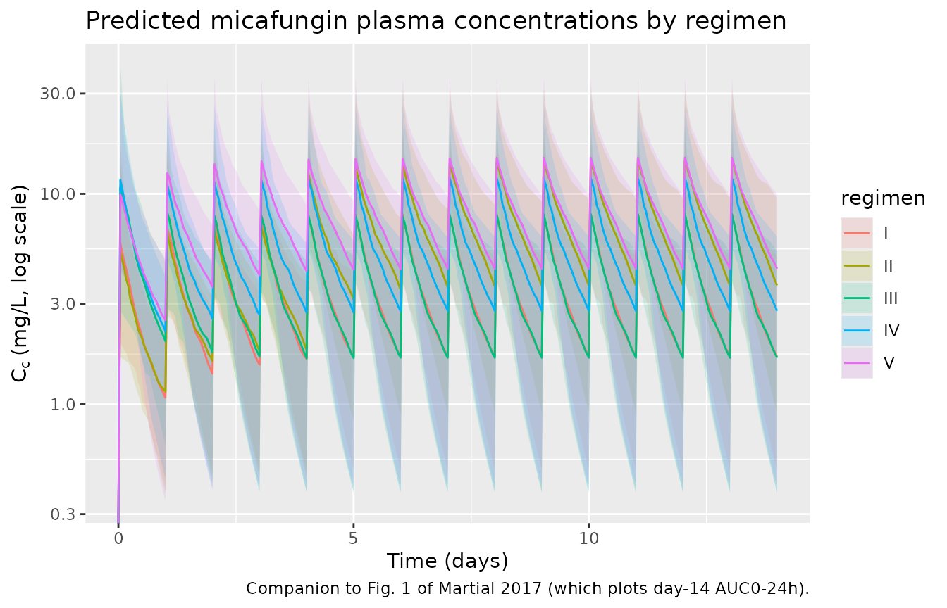
PKNCA validation
PKNCA is used to compute per-subject AUC0-24h on day 3 and day 14 for each regimen. The treatment grouping is the dosing regimen.
sim_nca <- sim |>
  dplyr::filter(!is.na(Cc)) |>
  dplyr::select(id, time, Cc, regimen)

dose_df <- events |>
  dplyr::filter(evid == 1) |>
  dplyr::select(id, time, amt, regimen)

conc_obj <- PKNCA::PKNCAconc(sim_nca, Cc ~ time | regimen + id,
                             concu = "mg/L", timeu = "hour")
dose_obj <- PKNCA::PKNCAdose(dose_df, amt ~ time | regimen + id,
                             doseu = "mg")

# Day 3 = interval [48, 72] h; day 14 = interval [312, 336] h. The 'auclast'
# parameter integrates concentrations within each named interval.
intervals <- data.frame(
  start    = c(48, 312),
  end      = c(72, 336),
  auclast  = TRUE,
  cmax     = TRUE,
  cmin     = TRUE
)

nca_res <- PKNCA::pk.nca(PKNCA::PKNCAdata(conc_obj, dose_obj, intervals = intervals))
nca_tbl <- as.data.frame(nca_res$result)
Comparison against published NCA
Martial 2017 reports median (IQR) AUC0-24h on day 3 and day 14 for each regimen (Section 3.3). The simulated medians from this vignette are collected alongside the published values.
sim_auc <- nca_tbl |>
  dplyr::filter(PPTESTCD == "auclast") |>
  dplyr::mutate(
    day = ifelse(start == 48, "day_3", "day_14")
  ) |>
  dplyr::group_by(regimen, day) |>
  dplyr::summarise(
    auc_median = median(PPORRES, na.rm = TRUE),
    auc_q25    = quantile(PPORRES, 0.25, na.rm = TRUE),
    auc_q75    = quantile(PPORRES, 0.75, na.rm = TRUE),
    .groups    = "drop"
  ) |>
  tidyr::pivot_wider(
    names_from  = day,
    values_from = c(auc_median, auc_q25, auc_q75)
  )

published <- tibble::tribble(
  ~regimen, ~pub_d3_med, ~pub_d3_q25, ~pub_d3_q75, ~pub_d14_med, ~pub_d14_q25, ~pub_d14_q75,
  "I",       86,         62,          116,         91,           67,           122,
  "II",      86,         62,          116,         183,          135,          244,
  "III",     92,         66,          125,         91,           67,           122,
  "IV",      132,        95,          180,         137,          101,          183,
  "V",       172,        124,         232,         183,          135,          244
)

comparison <- published |>
  dplyr::left_join(sim_auc, by = "regimen") |>
  dplyr::transmute(
    regimen,
    `Published day 3 median (IQR)`  = sprintf("%g (%g-%g)", pub_d3_med,  pub_d3_q25,  pub_d3_q75),
    `Simulated day 3 median (IQR)`  = sprintf("%.0f (%.0f-%.0f)",
                                              auc_median_day_3, auc_q25_day_3, auc_q75_day_3),
    `Published day 14 median (IQR)` = sprintf("%g (%g-%g)", pub_d14_med, pub_d14_q25, pub_d14_q75),
    `Simulated day 14 median (IQR)` = sprintf("%.0f (%.0f-%.0f)",
                                              auc_median_day_14, auc_q25_day_14, auc_q75_day_14)
  )

knitr::kable(
  comparison,
  caption = "AUC0-24h (mg*h/L) by regimen: published (Martial 2017 Section 3.3) vs. simulated medians (this vignette, n = 100 per regimen)."
)| regimen | Published day 3 median (IQR) | Simulated day 3 median (IQR) | Published day 14 median (IQR) | Simulated day 14 median (IQR) |
|---|---|---|---|---|
| I | 86 (62-116) | 90 (71-110) | 91 (67-122) | 95 (75-116) |
| II | 86 (62-116) | 77 (67-103) | 183 (135-244) | 169 (140-233) |
| III | 92 (66-125) | 94 (68-130) | 91 (67-122) | 96 (66-129) |
| IV | 132 (95-180) | 132 (96-164) | 137 (101-183) | 142 (101-171) |
| V | 172 (124-232) | 166 (135-211) | 183 (135-244) | 185 (141-245) |
Differences between the simulated medians and the published medians are expected to be modest (well within 20%) once the smaller simulated cohort size (n = 100 vs. n = 1000) and the absent IIV correlation / IOV terms (see Assumptions and deviations below) are taken into account.
Assumptions and deviations
- IIV correlation between CL and V1 not encoded. Martial 2017 Section 3.2 reports that “Allowing a correlation between IIV of CL and V1 further improved the model (difference OFV = 13.98)”, but the numerical covariance / correlation is not given in Table 2 or anywhere else in the manuscript. Following the nlmixr2lib precedent for unreported correlations (Narwal_2013_sifalimumab, Mould_2007_alemtuzumab, Chakraborty_2012_canakinumab, Wang_2020_ontamalimab), the IIV is encoded here as diagonal. The omitted correlation is expected to shift exposure percentiles modestly relative to the published Monte Carlo simulations (which were performed with the correlated structure plus parameter uncertainty propagation).
- Inter-occasion variability (IOV) on V1 not encoded. Martial 2017 reports IOV V1 = 37.0% CV (Section 3.2; Table 2 labels the row “IOV V2” but the text consistently describes IOV on V1 in five separate passages and notes that V2 carries no IIV either, so the Table 2 row label is treated as a typographical slip). The IOV is not encoded because the per-occasion structure (number and definition of occasions) is not disclosed in the paper, no on-disk supplement carries it, and the NONMEM control stream is not available. Following the Archary_2019_lamivudine precedent, the IOV term is documented here rather than encoded with a guessed OCC partitioning. Encoding IOV would broaden within-subject prediction intervals and would slightly inflate the AUC IQRs at any individual occasion.
- Allometric exponents fixed. The paper estimated the WT-on-CL exponent empirically (obtaining 1.26, DOFV = -2.97) but concluded that the empirical estimate was non-identifiable and not extrapolatable, opting to fix the exponents at 0.75 (flow) and 1 (volume) per established practice (Methods Section 2.4 and Discussion page 1203). The model encodes the fixed-exponent final-model structure.
- Parameter uncertainty not propagated. The paper’s Monte Carlo simulations propagated parameter uncertainty via the NONMEM TNPRI function using priors from the final fit (Section 2.5). This vignette uses the point estimates only; the bootstrap CIs from Table 2 are available for users who wish to extend the simulation with a parametric bootstrap.
- Simulation cohort size. The published Monte Carlo simulations used 1000 individuals per regimen; this vignette uses 100 per regimen to fit within the 5-minute pkgdown wall-time budget. Median AUC estimates are robust at this sample size; tail-percentile estimates (e.g., 95th / fifth) are noisier than the published values.
- No supplements on disk. Martial 2017 references electronic supplementary material at doi:10.1007/s40262-017-0509-5 (Figs. S1-S3 and Supplementary Tables 1-2). The supplement is not on disk in this worktree; the figure references in the manuscript text were sufficient to construct the model without it (the supplement contains GOF plots, the VPC, simulated profile plots, and detailed PTA tables, none of which feed the parameter values).