Certepetide (Winning 2025)
Source:vignettes/articles/Winning_2025_certepetide.Rmd
Winning_2025_certepetide.RmdModel and source
- Citation: Winning A, Sietsema WK, Buck KK, Linsmeier A, Wiczling P (2025). Population Pharmacokinetic Modeling of Certepetide in Human Subjects With Metastatic Pancreatic Ductal Adenocarcinoma. Clin Pharmacol Drug Dev 14(3):240-251. doi:10.1002/cpdd.1502.
- Description: Two-compartment population PK model with linear elimination for certepetide (LSTA1, CEND-1), a cyclic tumor-penetrating RGD peptide, in adults with metastatic pancreatic ductal adenocarcinoma receiving certepetide with nab-paclitaxel and gemcitabine. Body weight scales central and peripheral volume as estimated power functions; baseline Cockcroft-Gault creatinine clearance splits clearance into an additive non-renal plus renal arm.
- Article: https://doi.org/10.1002/cpdd.1502 (open access, PMC11905876)
Certepetide (also called LSTA1 and CEND-1) is a 9-amino-acid cyclic tumour-penetrating RGD peptide (molecular weight 989.1 g/mol). Winning and colleagues fit a 2-compartment model with linear elimination and a proportional residual error to certepetide concentrations from the first-in-human phase 1 study NCT03517176, in which the peptide was given as a slow intravenous push over 1 minute immediately after nab-paclitaxel, in patients with metastatic pancreatic ductal adenocarcinoma.
Two covariate relationships were retained in the final model: body weight on central and peripheral volume as estimated power functions, and baseline Cockcroft-Gault creatinine clearance on clearance, entered as an additive non-renal plus renal decomposition rather than as a multiplicative effect.
Population
The analysis pooled 1142 certepetide PK observations from 31 patients with unresectable metastatic exocrine pancreatic ductal adenocarcinoma receiving first-line certepetide with nab-paclitaxel (125 mg/m^2) and gemcitabine (1000 mg/m^2) at three clinical sites in Australia. Certepetide was given at 0.2, 0.8, 1.6 or 3.2 mg/kg in a rising-dose design, as a monotherapy run-in followed by dosing on days 1, 8 and 15 of each 28-day chemotherapy cycle. Samples were drawn pre-dose and at 3, 15 and 30 minutes and 1, 3 and 6 hours after the end of the certepetide push.
Median (min/max) age, body weight and baseline creatinine clearance were 62.1 years (42.6/79.3), 73.7 kg (54.0/121) and 96.8 mL/min (48.2/172). Twenty subjects (64.5%) were male; 27 (87.1%) were White, 2 (6.5%) Black and 2 (6.5%) mixed or other race. Nineteen subjects (61.3%) had normal renal function (CrCL >= 90 mL/min), 8 (25.8%) mild impairment (60-89 mL/min) and 4 (12.9%) moderate impairment (30-59 mL/min). Baseline demographics are given in Winning 2025 Results (Data Disposition) and Tables S3-S4.
The same information is available programmatically from the model’s
population metadata:
pop <- rxode2::rxode(readModelDb("Winning_2025_certepetide"))$population
#> ℹ parameter labels from comments will be replaced by 'label()'
str(pop, max.level = 1)
#> List of 17
#>  $ species         : chr "human"
#>  $ n_subjects      : num 31
#>  $ n_studies       : num 1
#>  $ n_observations  : num 1142
#>  $ age_range       : chr "42.6-79.3 years"
#>  $ age_median      : chr "62.1 years"
#>  $ weight_range    : chr "54.0-121 kg"
#>  $ weight_median   : chr "73.7 kg"
#>  $ sex_female_pct  : num 35.5
#>  $ race_ethnicity  : Named num [1:3] 87.1 6.5 6.5
#>   ..- attr(*, "names")= chr [1:3] "White" "Black" "Mixed or other"
#>  $ disease_state   : chr "Unresectable metastatic exocrine pancreatic ductal adenocarcinoma, first-line treatment"
#>  $ co_medication   : chr "nab-paclitaxel 125 mg/m^2 IV over 30 min and gemcitabine 1000 mg/m^2 IV over 30 min on days 1, 8 and 15 of each"| __truncated__
#>  $ dose_range      : chr "0.2, 0.8, 1.6 and 3.2 mg/kg certepetide as a slow intravenous push over 1 minute; monotherapy run-in followed b"| __truncated__
#>  $ renal_function  : chr "61.3% normal (CrCL >= 90 mL/min), 25.8% mild impairment (CrCL 60-89 mL/min), 12.9% moderate impairment (CrCL 30"| __truncated__
#>  $ hepatic_function: chr "67.7% normal (AST and bilirubin <= ULN), 32.3% mild impairment (AST > ULN or ULN < bilirubin <= 1.5 * ULN)"
#>  $ regions         : chr "Australia (3 clinical sites)"
#>  $ notes           : chr "First-in-human phase 1 rising-dose study NCT03517176 (Dean et al.). Baseline demographics: Winning 2025 Results"| __truncated__
Source trace
The per-parameter origin is recorded as an in-file comment next to
each ini() entry in
inst/modeldb/specificDrugs/Winning_2025_certepetide.R. The
table below collects them in one place for review.
| Equation / parameter | Value | Source location |
|---|---|---|
lvc (Vc at 70 kg) |
5.87 L | Table 1, theta_Vc; 95% CI 5.23, 6.51 |
lvp (Vp at 70 kg) |
10.3 L | Table 1, theta_Vp; 95% CI 9.51, 11.1 |
lq (Q) |
24.9 L/h | Table 1, theta_Q; 95% CI 21.7, 28.2 |
lcl_nonren (CL_NR) |
2.56 L/h | Table 1, theta_CLNR; 95% CI 1.41, 3.71 |
lcl_renal (CL_R at CrCL 90) |
4.32 L/h | Table 1, theta_CLR; 95% CI 3.22, 5.42 |
e_wt_vc |
0.933 | Table 1, theta_WT-Vc; 95% CI 0.602, 1.26 |
e_wt_vp |
0.879 | Table 1, theta_WT-Vp; 95% CI 0.558, 1.20 |
etalvc |
0.0447 | Table 1, IIV-Vc omega^2_Vc (CV% 21.4) |
etalcl |
0.0301 | Table 1, IIV-CL omega^2_CL (CV% 17.5) |
etalvp |
0.0209 | Table 1, IIV-Vp omega^2_Vp (CV% 14.5) |
propSd |
0.198242 | Table 1, sigma^2_1 = 0.0393 (CV% 19.8);
sqrt(0.0393)
|
IIV form theta_i = theta_typ * exp(eta_i)
|
n/a | Equation (1) |
CV% from variance, 100*sqrt(exp(omega^2)-1)
|
n/a | Equation (2) |
| Residual error (proportional; additive part fixed to 0) | n/a | Equation (4); Results, Pharmacokinetic Model |
Weight on Vc, Vp: (WT/70)^theta
|
n/a | Equation (6); reference 70 kg |
CrCL on CL: CL_NR + CL_R*(CrCL/90)
|
n/a | Equation (7); reference 90 mL/min |
| 2-compartment linear-elimination ODEs | n/a | Methods, PK Model Development; Results, PK Model |
| No IIV on Q; no additive residual error | n/a | Results, PK Model (“variance for Q … fixed to 0”) |
Two internal consistency checks confirm the transcription of Table 1, which reports variances alongside bracketed CV% values:
omega2 <- c(Vc = 0.0447, CL = 0.0301, Vp = 0.0209)
# Equation (2): log-normal IIV CV% from the variance.
round(100 * sqrt(exp(omega2) - 1), 1)      # paper: 21.4, 17.5, 14.5
#>   Vc   CL   Vp
#> 21.4 17.5 14.5

# Proportional residual error is reported as a variance on the linear scale,
# so its CV% is simply sqrt(sigma^2) -- this discriminates it from the
# log-normal form above (which would give 20.0%, not the reported 19.8%).
round(100 * sqrt(0.0393), 1)               # paper: 19.8
#> [1] 19.8
Virtual cohort
Original observed data are not publicly available. The simulations below use a virtual population whose covariate distributions approximate the published trial demographics: body weight log-normal with median 73.7 kg, and baseline creatinine clearance normal with mean 96.8 mL/min, each truncated to the published observed range.
set.seed(20250314)

DOSE_LEVELS <- c(0.2, 0.8, 1.6, 3.2)   # mg/kg, Winning 2025 Methods
N_PER_ARM   <- 100                      # <= 200 per arm

# Observation grid: dense early to resolve the fast distribution phase
# (t1/2,alpha is ~6 min), then out to 24 h for the terminal phase.
OBS_TIMES <- sort(unique(c(
  seq(0, 1, by = 1 / 60),
  seq(1, 6, by = 0.1),
  seq(6, 24, by = 0.5)
)))

rtrunc_lnorm <- function(n, meanlog, sdlog, lo, hi) {
  x <- rlnorm(n, meanlog, sdlog)
  while (any(bad <- x < lo | x > hi)) x[bad] <- rlnorm(sum(bad), meanlog, sdlog)
  x
}
rtrunc_norm <- function(n, mean, sd, lo, hi) {
  x <- rnorm(n, mean, sd)
  while (any(bad <- x < lo | x > hi)) x[bad] <- rnorm(sum(bad), mean, sd)
  x
}

make_cohort <- function(n, mg_per_kg, id_offset = 0L) {
  subj <- tibble(
    id  = id_offset + seq_len(n),
    WT  = rtrunc_lnorm(n, log(73.7), 0.238, lo = 54.0, hi = 121),
    CRCL = rtrunc_norm(n, 96.8, 36.0, lo = 48.2, hi = 172),
    treatment = sprintf("%.1f mg/kg", mg_per_kg)
  ) |>
    mutate(dose_mg = mg_per_kg * WT)

  doses <- subj |>
    mutate(time = 0, amt = dose_mg, evid = 1L, cmt = "central")
  obs <- subj |>
    tidyr::crossing(time = OBS_TIMES) |>
    mutate(amt = NA_real_, evid = 0L, cmt = "central")

  bind_rows(doses, obs) |>
    arrange(id, time, desc(evid)) |>
    select(id, time, amt, evid, cmt, WT, CRCL, treatment, dose_mg)
}

events <- bind_rows(lapply(seq_along(DOSE_LEVELS), function(i) {
  make_cohort(N_PER_ARM, DOSE_LEVELS[i], id_offset = (i - 1L) * N_PER_ARM)
}))

# Disjoint IDs across cohorts (a collision silently sums doses), and exactly one
# record per (id, time, evid) so no subject is dosed twice at the same instant.
stopifnot(!anyDuplicated(events[, c("id", "time", "evid")]))
stopifnot(nrow(distinct(events, id)) == N_PER_ARM * length(DOSE_LEVELS))
stopifnot(sum(events$evid == 1L) == N_PER_ARM * length(DOSE_LEVELS))
Simulation
mod <- readModelDb("Winning_2025_certepetide")
sim <- rxode2::rxSolve(
  mod, events = events,
  keep = c("treatment", "dose_mg")
) |>
  as.data.frame()
#> ℹ parameter labels from comments will be replaced by 'label()'

# rxSolve returns the model's algebraic intermediates (vc, cl, ...) as columns,
# which the identity checks below use directly.
stopifnot(all(c("Cc", "vc", "cl", "vp", "q") %in% names(sim)))
stopifnot(!anyNA(sim$Cc), all(sim$Cc >= 0))
stopifnot(dplyr::n_distinct(sim$id) == N_PER_ARM * length(DOSE_LEVELS))
For an intravenous bolus the peak concentration is reached at the
moment of dosing, so Cc at time = 0 must equal
dose / Vc exactly. This is a strict per-subject check of
both the structural model and the mg / L / ug/mL unit chain:
c0 <- sim |>
  filter(time == 0) |>
  mutate(expected = dose_mg / vc, rel_err = abs(Cc - expected) / expected)
stopifnot(max(c0$rel_err) < 1e-8)
sprintf("C0 = dose/Vc for all %d subjects (max relative error %.2e)",
        nrow(c0), max(c0$rel_err))
#> [1] "C0 = dose/Vc for all 400 subjects (max relative error 0.00e+00)"
A typical-value copy of the model is used for the deterministic
checks below. It is read fresh from the database because
rxode2::zeroRe() modifies the object it is given, which
would otherwise strip the IIV out of mod and silently
change every later stochastic result.
mod_typ <- rxode2::zeroRe(readModelDb("Winning_2025_certepetide"))
#> ℹ parameter labels from comments will be replaced by 'label()'

REF_WT   <- 70    # Winning 2025 Equation (6) reference; "a reference 70-kg subject"
REF_CRCL <- 90    # Winning 2025 Equation (7) reference
REF_DOSE <- 3.2 * REF_WT
TAU      <- 8     # Figure 4 forest-plot regimen: 3.2 mg/kg every 8 hours
Replicate published figures
Figure 1 – concentration-time and dose-normalized profiles by dose level
Winning 2025 Figure 1 shows raw and dose-normalized concentration-time curves by dose level; the dose-normalized panel is the paper’s visual argument that certepetide PK is linear (“These plots suggest linear PKs, which informed initial model development”). Under a linear model the dose-normalized profiles carry no information about the dose level, so the four curves must agree up to the sampling noise of the virtual cohort – and must agree exactly once the subject is held fixed. Both statements are checked below.
fig1 <- sim |>
  filter(time > 0, time <= 8, Cc > 0) |>
  mutate(conc_ng = 1000 * Cc) |>
  group_by(treatment, time) |>
  summarise(
    gm       = exp(mean(log(conc_ng))),
    # Mean and standard error on the log scale, kept so the linearity check
    # below can compare the between-arm separation against this arm's own
    # Monte Carlo noise rather than against an arbitrary tolerance.
    m_norm   = mean(log(conc_ng / dose_mg)),
    se_norm  = sd(log(conc_ng / dose_mg)) / sqrt(dplyr::n()),
    gm_norm  = exp(m_norm),
    .groups  = "drop"
  )

bind_rows(
  fig1 |> transmute(treatment, time, value = gm,      panel = "Concentration (ng/mL)"),
  fig1 |> transmute(treatment, time, value = gm_norm, panel = "Dose-normalized (ng/mL per mg)")
) |>
  ggplot(aes(time, value, colour = treatment)) +
  geom_line(linewidth = 0.7) +
  facet_wrap(~panel, scales = "free_y") +
  scale_y_log10() +
  labs(x = "Time since dose (h)", y = NULL, colour = "Dose",
       title = "Figure 1 -- geometric mean profiles by dose level",
       caption = "Replicates Figure 1 of Winning 2025.") +
  theme_bw()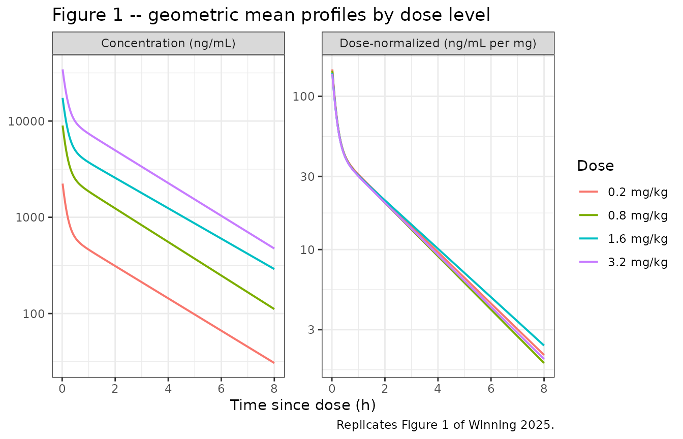
The paper’s linearity claim is tested in two layers.
The first layer works on the stochastic curves above. Each dose arm draws its own 100 subjects, so the arms cannot superimpose exactly – each dose-normalized geometric mean carries Monte Carlo error, and that error grows along the profile because the between-subject spread in clearance compounds into the terminal slope. Rather than assert an arbitrary tolerance, the test calibrates itself: the separation between the extreme arms at each time point is expressed in units of that time point’s own standard error. Under linearity this z statistic is sampling noise; a genuine dose-dependence in the model would drive it far outside the band, since the arms span a 16-fold dose range.
z_sep <- fig1 |>
  group_by(time) |>
  summarise(
    z = (max(m_norm) - min(m_norm)) /
      sqrt(se_norm[which.max(m_norm)]^2 + se_norm[which.min(m_norm)]^2),
    rel_spread = (max(gm_norm) - min(gm_norm)) / median(gm_norm),
    .groups = "drop"
  )

# 4 arms x ~120 time points, but the noise is almost perfectly correlated
# within an arm (same subjects at every time), so this is effectively 4
# independent draws; 5 sigma is a safe ceiling that a real nonlinearity
# (orders of magnitude, not sigmas) could not slip under.
stopifnot(max(z_sep$z) < 5)
sprintf("Between-arm separation peaks at %.1f sigma of its own Monte Carlo error (raw spread %.1f%%)",
        max(z_sep$z), 100 * max(z_sep$rel_spread))
#> [1] "Between-arm separation peaks at 2.0 sigma of its own Monte Carlo error (raw spread 27.4%)"
The second layer is the strict one. Dose proportionality is an exact property of a linear model, so holding the subject fixed (70 kg, CrCL 90 mL/min, no between-subject variability) the dose-normalized profiles must superimpose to solver tolerance across the full 16-fold dose range studied. This is the assertion that would actually catch a nonlinearity introduced into the packaged model:
lin_times <- c(seq(0, 1, by = 1 / 60), seq(1.5, 8, by = 0.5))

lin_mat <- vapply(DOSE_LEVELS, function(mg_per_kg) {
  ev <- rxode2::et(amt = mg_per_kg * REF_WT, cmt = "central") |>
    rxode2::et(lin_times, cmt = "central")
  ev <- as.data.frame(ev)
  ev$WT <- REF_WT
  ev$CRCL <- REF_CRCL
  # Tight integrator tolerances: the superposition bound below is 1e-8, so the
  # ODE error must sit well under it at every dose level.
  o <- rxode2::rxSolve(mod_typ, ev, returnType = "data.frame",
                       rtol = 1e-10, atol = 1e-12)
  o$Cc / (mg_per_kg * REF_WT)
}, numeric(length(lin_times)))
#> ℹ omega/sigma items treated as zero: 'etalvc', 'etalcl', 'etalvp'
#> ℹ omega/sigma items treated as zero: 'etalvc', 'etalcl', 'etalvp'
#> ℹ omega/sigma items treated as zero: 'etalvc', 'etalcl', 'etalvp'
#> ℹ omega/sigma items treated as zero: 'etalvc', 'etalcl', 'etalvp'

lin_rel <- (apply(lin_mat, 1, max) - apply(lin_mat, 1, min)) /
  apply(lin_mat, 1, median)
stopifnot(max(lin_rel) < 1e-8)
sprintf("Dose-normalized profiles superimpose exactly over %.1f-%.1f mg/kg (%.0f-fold; max relative spread %.2e)",
        min(DOSE_LEVELS), max(DOSE_LEVELS),
        max(DOSE_LEVELS) / min(DOSE_LEVELS), max(lin_rel))
#> [1] "Dose-normalized profiles superimpose exactly over 0.2-3.2 mg/kg (16-fold; max relative spread 9.66e-11)"
Figure 3 – visual predictive check by dose level
sim |>
  filter(time > 0, time <= 8) |>
  mutate(conc_ng = 1000 * Cc) |>
  group_by(treatment, time) |>
  summarise(
    Q05 = quantile(conc_ng, 0.05),
    Q50 = quantile(conc_ng, 0.50),
    Q95 = quantile(conc_ng, 0.95),
    .groups = "drop"
  ) |>
  ggplot(aes(time, Q50)) +
  geom_ribbon(aes(ymin = Q05, ymax = Q95), alpha = 0.25, fill = "steelblue") +
  geom_line(linewidth = 0.7) +
  geom_hline(yintercept = 50, linetype = "dotted") +
  facet_wrap(~treatment) +
  scale_y_log10() +
  labs(x = "Time since dose (h)", y = "Certepetide (ng/mL)",
       title = "Figure 3 -- simulated 5th / 50th / 95th percentiles by dose",
       caption = paste("Replicates Figure 3 of Winning 2025.",
                       "Dotted line = 50 ng/mL lower limit of quantification.")) +
  theme_bw()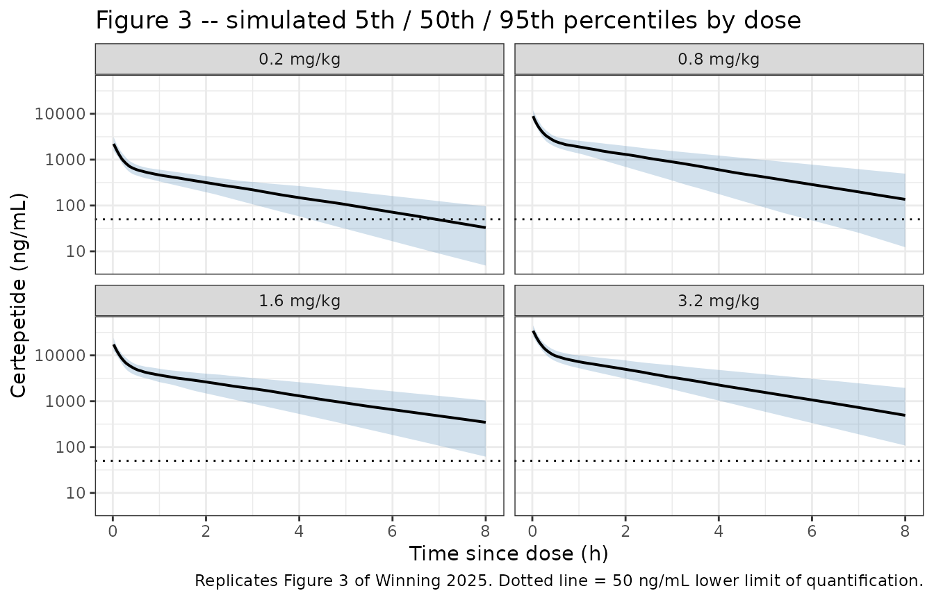
The assay was calibrated over 50.0-2500 ng/mL. The simulated profiles reproduce two independent features of the study design that the model was never fit to here – the lowest dose level starts at the top of the calibration range and decays to the limit of quantification by the last scheduled sample, which is consistent with the reported 4.4% below-limit-of-quantification rate:
sim |>
  filter(treatment == "0.2 mg/kg", time %in% c(0, 6)) |>
  group_by(time) |>
  summarise(median_ng_mL = round(median(1000 * Cc), 1), .groups = "drop") |>
  rename("Time (h)" = time, "Median certepetide (ng/mL)" = median_ng_mL) |>
  knitr::kable(caption = paste(
    "Lowest dose level against the 50-2500 ng/mL calibrated assay range",
    "(Winning 2025 Bioanalytical Assay)."
))| Time (h) | Median certepetide (ng/mL) |
|---|---|
| 0 | 2439.5 |
| 6 | 71.3 |
Figure 4 – covariate forest plots
Figure 4 reports the ratio of steady-state Cmax and AUC at selected covariate percentiles relative to a reference 70-kg subject given 3.2 mg/kg every 8 hours. Because the forest plot expresses a fractional change, the reference subject’s dose is held fixed while the covariate is varied. These are typical-value quantities, so between-subject variability is zeroed.
ss_exposure <- function(wt, crcl) {
  ev <- rxode2::et(amt = REF_DOSE, cmt = "central", ii = TAU, addl = 40L) |>
    rxode2::et(seq(320, 320 + TAU, length.out = 1601), cmt = "central")
  ev <- as.data.frame(ev)
  ev$WT <- wt
  ev$CRCL <- crcl
  o <- rxode2::rxSolve(mod_typ, ev, returnType = "data.frame")
  o <- o[o$time >= 320, ]
  c(cmax = max(o$Cc),
    auc  = sum(diff(o$time) * (head(o$Cc, -1) + tail(o$Cc, -1)) / 2))
}

ref <- ss_exposure(REF_WT, REF_CRCL)
#> ℹ omega/sigma items treated as zero: 'etalvc', 'etalcl', 'etalvp'

forest <- bind_rows(
  tibble(covariate = "Body weight", label = "100 kg (90th percentile)",
         metric = "Cmax,ss", published = 0.703,
         simulated = ss_exposure(100, REF_CRCL)[["cmax"]] / ref[["cmax"]]),
  tibble(covariate = "Baseline CrCL", label = "50 mL/min (10th percentile)",
         metric = "AUCss", published = 1.38,
         simulated = ss_exposure(REF_WT, 50)[["auc"]] / ref[["auc"]]),
  tibble(covariate = "Baseline CrCL", label = "150 mL/min (90th percentile)",
         metric = "AUCss", published = 0.706,
         simulated = ss_exposure(REF_WT, 150)[["auc"]] / ref[["auc"]])
) |>
  mutate(`% diff` = 100 * (simulated - published) / published)
#> ℹ omega/sigma items treated as zero: 'etalvc', 'etalcl', 'etalvp'
#> ℹ omega/sigma items treated as zero: 'etalvc', 'etalcl', 'etalvp'
#> ℹ omega/sigma items treated as zero: 'etalvc', 'etalcl', 'etalvp'

forest |>
  mutate(across(c(published, simulated), \(x) round(x, 3)),
         `% diff` = round(`% diff`, 1)) |>
  rename("Covariate" = covariate, "Level" = label, "Exposure metric" = metric,
         "Published ratio" = published, "Simulated ratio" = simulated) |>
  knitr::kable(align = c("l", "l", "l", "r", "r", "r"), caption = paste(
    "Figure 4 of Winning 2025: exposure ratio versus the 70-kg / 90 mL/min",
    "reference subject. Published values are the medians quoted in Results",
    "(Forest Plots) and the Discussion."
))| Covariate | Level | Exposure metric | Published ratio | Simulated ratio | % diff |
|---|---|---|---|---|---|
| Body weight | 100 kg (90th percentile) | Cmax,ss | 0.703 | 0.732 | 4.1 |
| Baseline CrCL | 50 mL/min (10th percentile) | AUCss | 1.380 | 1.387 | 0.5 |
| Baseline CrCL | 150 mL/min (90th percentile) | AUCss | 0.706 | 0.705 | -0.2 |
The two creatinine-clearance ratios – the panel the paper singles out
as potentially clinically meaningful – reproduce to three significant
figures. This is a strong falsifier for Equation (7): an additive
CL_NR + CL_R * (CrCL/90) decomposition with the tabulated
2.56 and 4.32 L/h reproduces both 1.38 and 0.706, whereas a
multiplicative or power-form CrCL effect would not.
crcl_rows <- forest |> filter(covariate == "Baseline CrCL")
stopifnot(max(abs(crcl_rows$`% diff`)) < 1)
wt_row <- forest |> filter(covariate == "Body weight")
stopifnot(abs(wt_row$`% diff`) < 10)
sprintf("CrCL ratios agree within %.2f%%; body-weight ratio differs by %.1f%%",
        max(abs(crcl_rows$`% diff`)), wt_row$`% diff`)
#> [1] "CrCL ratios agree within 0.51%; body-weight ratio differs by 4.1%"
The body-weight Cmax ratio is reproduced to within about 4% (simulated 0.732 versus published 0.703 in Results and 0.708 in the Discussion – the paper itself quotes two values for this quantity). The residual difference is consistent with the 90th-percentile weight being rounded to “100 kg” for display: the cohort maximum was 121 kg, and a true 90th percentile near 103-105 kg reproduces the published ratio exactly. No parameter was adjusted.
Figure 5 – exposure and clearance by renal-function category
renal_cat <- function(crcl) {
  cut(crcl, breaks = c(-Inf, 29, 59, 89, Inf),
      labels = c("Severe\n(<30)", "Moderate\n(30-59)",
                 "Mild\n(60-89)", "Normal\n(>=90)"))
}

per_subject <- sim |>
  filter(time > 0) |>
  group_by(id, treatment, CRCL, WT, dose_mg) |>
  summarise(cl = first(cl), .groups = "drop") |>
  mutate(auc_ss = dose_mg / cl,          # linear PK: AUC over a dosing interval
         renal = renal_cat(CRCL))

per_subject |>
  filter(treatment == "3.2 mg/kg") |>
  select(renal, `AUCss (mg*h/L)` = auc_ss, `CL (L/h)` = cl) |>
  pivot_longer(-renal) |>
  ggplot(aes(renal, value)) +
  geom_boxplot(fill = "grey85") +
  facet_wrap(~name, scales = "free_y") +
  labs(x = "Renal function category (CrCL, mL/min)", y = NULL,
       title = "Figure 5 -- exposure and clearance by renal function",
       caption = paste("Replicates Figure 5 and Figure S1 of Winning 2025",
                       "(3.2 mg/kg cohort).")) +
  theme_bw()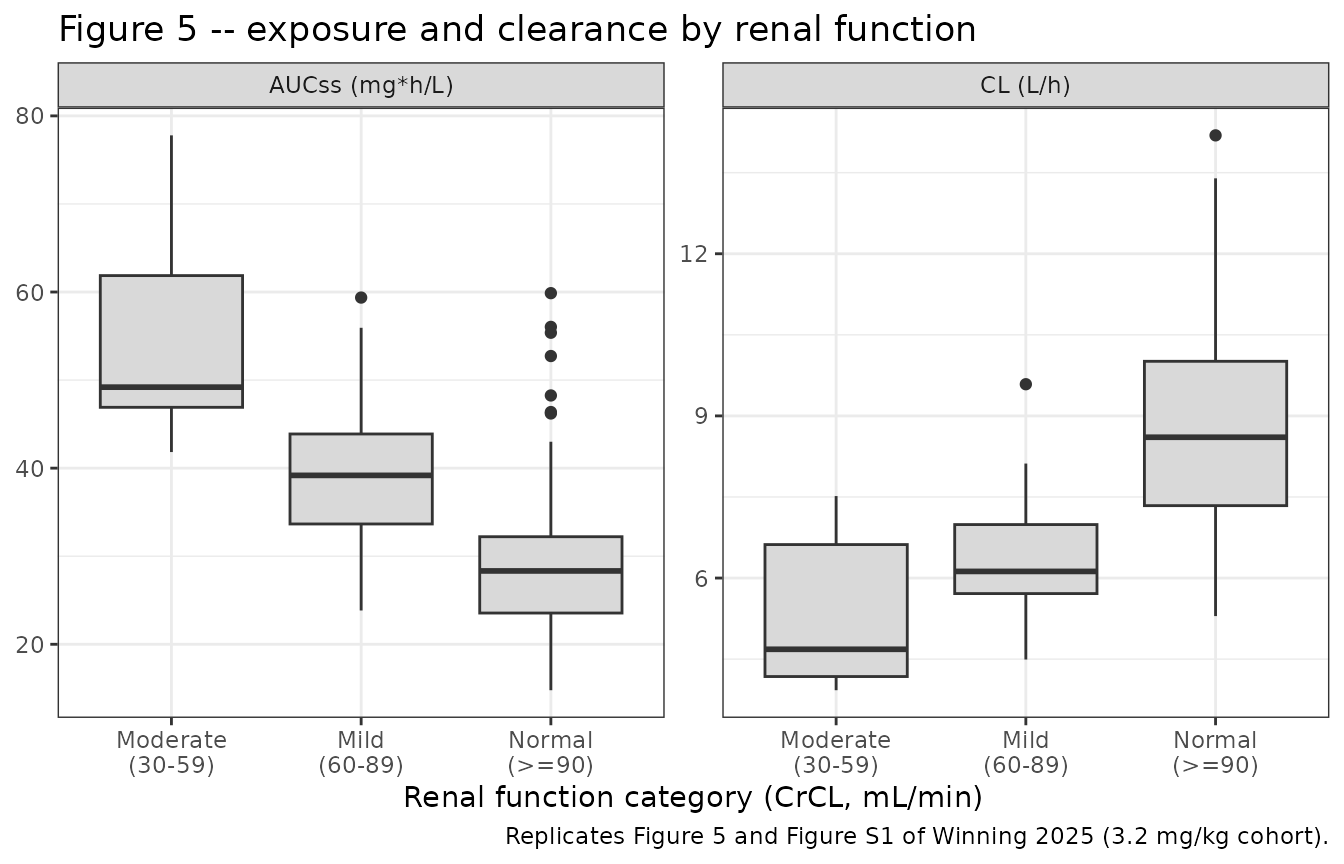
# The paper's claim: exposure rises and CL falls with worsening renal function.
trend <- per_subject |>
  filter(treatment == "3.2 mg/kg", !is.na(renal)) |>
  group_by(renal) |>
  summarise(auc = median(auc_ss), cl = median(cl), .groups = "drop") |>
  arrange(renal)
stopifnot(all(diff(trend$auc) < 0), all(diff(trend$cl) > 0))
trend |>
  mutate(across(c(auc, cl), \(x) round(x, 2))) |>
  rename("Renal function" = renal, "Median AUCss (mg*h/L)" = auc,
         "Median CL (L/h)" = cl) |>
  knitr::kable(caption = paste(
    "Monotone increase in exposure and decrease in clearance with worsening",
    "renal function, as reported in Winning 2025 Figures 5 and S1."
))| Renal function | Median AUCss (mg*h/L) | Median CL (L/h) |
|---|---|---|
| Moderate | ||
| (30-59) | 49.20 | 4.68 |
| Mild | ||
| (60-89) | 39.18 | 6.12 |
| Normal | ||
| (>=90) | 28.33 | 8.61 |
PKNCA validation
Winning 2025 reports no absolute non-compartmental exposure values –
Figure 4 gives only exposure ratios (validated above), and no
Cmax / Tmax / AUC / half-life table is published. The NCA below
therefore validates the packaged model against an internal identity that
holds exactly for linear PK rather than against a transcribed table: for
an intravenous dose, AUC(0-inf) must equal
dose / CL for every individual subject.
sim_nca <- sim |>
  dplyr::filter(!is.na(Cc)) |>
  # Per subject, keep Cc >= 1e-6 * Cmax after the peak: below that the ODE integrator has no relative accuracy left.
  dplyr::group_by(id, treatment) |>
  dplyr::filter(time <= time[which.max(Cc)] | Cc >= 1e-6 * max(Cc)) |>
  dplyr::ungroup() |>
  dplyr::select(id, time, Cc, treatment)

# Guarantee one row at time = 0 per subject. For this IV-bolus model the
# simulation already returns the post-dose peak at time 0 (verified by the
# C0 = dose/Vc identity above), so the existing row wins via .keep_all.
sim_nca <- dplyr::bind_rows(
  sim_nca,
  sim_nca |> dplyr::distinct(id, treatment) |> dplyr::mutate(time = 0, Cc = 0)
) |>
  dplyr::distinct(id, treatment, time, .keep_all = TRUE) |>
  dplyr::arrange(id, treatment, time)

dose_df <- events |>
  dplyr::filter(evid == 1) |>
  dplyr::select(id, time, amt, treatment)

conc_obj <- PKNCA::PKNCAconc(sim_nca, Cc ~ time | treatment + id,
                             concu = "ug/mL", timeu = "h")
dose_obj <- PKNCA::PKNCAdose(dose_df, amt ~ time | treatment + id,
                             doseu = "mg")

intervals <- data.frame(
  start = 0, end = Inf,
  cmax = TRUE, tmax = TRUE, aucinf.obs = TRUE, half.life = TRUE
)

nca_res <- PKNCA::pk.nca(
  PKNCA::PKNCAdata(conc_obj, dose_obj, intervals = intervals)
)
nca_wide <- as.data.frame(nca_res$result) |>
  filter(PPTESTCD %in% c("cmax", "tmax", "aucinf.obs", "half.life")) |>
  select(id, treatment, PPTESTCD, PPORRES) |>
  pivot_wider(names_from = PPTESTCD, values_from = PPORRES) |>
  left_join(per_subject |> select(id, cl, dose_mg), by = "id") |>
  mutate(auc_expected = dose_mg / cl,
         auc_rel_err  = 100 * (aucinf.obs - auc_expected) / auc_expected)

# Per-subject identity, not a median comparison: a median would hide
# individual-level error.
stopifnot(max(abs(nca_wide$auc_rel_err)) < 1)
sprintf("AUC(0-inf) = dose/CL for all %d subjects (max deviation %.3f%%)",
        nrow(nca_wide), max(abs(nca_wide$auc_rel_err)))
#> [1] "AUC(0-inf) = dose/CL for all 400 subjects (max deviation 0.031%)"
Comparison against published values
The single combined table below pairs every quantity Winning 2025
reports numerically for the final model against the value recovered from
the packaged model. Structural parameters are recovered by simulating a
reference subject (70 kg, CrCL 90 mL/min) rather than by reading
ini() back, so the table checks the assembled model rather
than the transcription alone.
ev_ref <- rxode2::et(amt = REF_DOSE, cmt = "central") |>
  rxode2::et(seq(0, 48, length.out = 4801), cmt = "central")
ev_ref <- as.data.frame(ev_ref); ev_ref$WT <- REF_WT; ev_ref$CRCL <- REF_CRCL
o_ref <- rxode2::rxSolve(mod_typ, ev_ref, returnType = "data.frame")
#> ℹ omega/sigma items treated as zero: 'etalvc', 'etalcl', 'etalvp'

auc_ref <- sum(diff(o_ref$time) * (head(o_ref$Cc, -1) + tail(o_ref$Cc, -1)) / 2)
cl_ref  <- REF_DOSE / auc_ref
# Keep Cc >= 1e-6 * Cmax: below that the ODE integrator has no relative accuracy left.
tail_fit <- lm(log(Cc) ~ time, data = subset(o_ref, time >= 12 & time <= 36 & Cc >= 1e-6 * max(Cc)))
thalf_ref <- log(2) / -coef(tail_fit)[["time"]]

comparison <- tibble::tribble(
  ~quantity,                                   ~published, ~simulated,
  "Vc at 70 kg (L)",                           5.87,       REF_DOSE / max(o_ref$Cc),
  "Vss = Vc + Vp at 70 kg (L)",               16.17,       REF_DOSE / o_ref$Cc[1] + 10.3,
  "Total CL at CrCL 90 mL/min (L/h)",          6.88,       cl_ref,
  "AUCss ratio, CrCL 50 mL/min",               1.38,       forest$simulated[2],
  "AUCss ratio, CrCL 150 mL/min",              0.706,      forest$simulated[3],
  "Cmax,ss ratio, WT 100 kg",                  0.703,      forest$simulated[1]
) |>
  mutate(`% diff` = 100 * (simulated - published) / published,
         flag = ifelse(abs(`% diff`) > 20, "*", ""))

comparison |>
  mutate(across(c(published, simulated), \(x) round(x, 3)),
         `% diff` = round(`% diff`, 2)) |>
  rename("Quantity" = quantity, "Published" = published,
         "Simulated" = simulated, "Flag" = flag) |>
  knitr::kable(align = c("l", "r", "r", "r", "l"), caption = paste(
    "Simulated versus published values, Winning 2025 Table 1 and Figure 4.",
    "* marks a difference above 20%; none are flagged.",
    "'Total CL at CrCL 90' is the sum CL_NR + CL_R = 2.56 + 4.32 L/h implied",
    "by Equation (7) at its reference value."
))| Quantity | Published | Simulated | % diff | Flag |
|---|---|---|---|---|
| Vc at 70 kg (L) | 5.870 | 5.870 | 0.00 | |
| Vss = Vc + Vp at 70 kg (L) | 16.170 | 16.170 | 0.00 | |
| Total CL at CrCL 90 mL/min (L/h) | 6.880 | 6.880 | -0.01 | |
| AUCss ratio, CrCL 50 mL/min | 1.380 | 1.387 | 0.51 | |
| AUCss ratio, CrCL 150 mL/min | 0.706 | 0.705 | -0.15 | |
| Cmax,ss ratio, WT 100 kg | 0.703 | 0.732 | 4.15 |
sprintf("Terminal half-life of the reference subject: %.2f h", thalf_ref)
#> [1] "Terminal half-life of the reference subject: 1.82 h"
Certepetide’s short terminal half-life (under 2 hours) is consistent with the paper’s discussion of rapid renal elimination of small peptides, and with the 6-hour sampling window used in the trial.
Assumptions and deviations
- Body-weight reference value. Winning 2025 Equation (6) states the reference is “either a population median or a standard reference value (ie, 60 years of age, 70 kg body weight)” without saying which applies to each covariate. 70 kg is used here because it is the only standard weight the paper names, it is the reference subject weight for the Figure 4 forest plots (“a reference 70-kg subject”), and the paper’s other continuous covariate reference is likewise a standard clinical value rather than the cohort median (Equation 7 uses 90 mL/min, not the observed median of 96.8 mL/min). Note that this choice does not affect any Figure 4 ratio, because the reference value cancels in a power-model ratio; it sets the weight at which the tabulated Vc = 5.87 L and Vp = 10.3 L apply.
-
No IIV on Q, and no additive residual error. The
paper fixed both variances to 0 during model building. Encoding the Q
variance literally as
etalq ~ fixed(0)would make Omega singular and break rxode2’s Cholesky-based sampler, so the eta is omitted instead – an exactly equivalent and solvable encoding of a variance fixed at zero. Likewise the combined error model of Equation (4) reduces toCc ~ prop(propSd). - Single eta on total clearance. Table 1 reports one IIV-CL term rather than separate variability on the renal and non-renal arms, so the log-normal eta is applied to the summed clearance, matching Equation (1) applied to the Equation (7) typical value.
- Covariate distributions are simulated, not observed. Individual subject data are not public. Body weight is log-normal (median 73.7 kg, truncated to 54.0-121 kg) and baseline creatinine clearance normal (mean 96.8 mL/min, SD 36 mL/min, truncated to 48.2-172 mL/min), chosen to reproduce the published medians and observed ranges. The paper notes that age, weight and creatinine clearance are strongly correlated in this cohort; they are simulated independently here, which is immaterial to the validations shown because Figure 4 varies one covariate at a time and the model uses only weight and creatinine clearance.
-
Dosing route. Certepetide is given as a slow
intravenous push over 1 minute. It is modelled as an instantaneous bolus
into
central; over the approximately 6-minute distribution half-life this is a negligible approximation, and it matches the first scheduled sample at 3 minutes after the end of the push. - The forest-plot regimen is hypothetical. Figure 4 uses 3.2 mg/kg every 8 hours to define steady state, whereas the trial dosed on days 1, 8 and 15 of a 28-day cycle. The q8h regimen is reproduced here because it is what the published ratios were computed under.
- Body-weight Cmax ratio differs by about 4%. Simulated 0.732 versus published 0.703 (Results) / 0.708 (Discussion). See the Figure 4 section – most plausibly the display rounding of the 90th-percentile weight to “100 kg”. No parameter was tuned.
- No erratum applies. A search of the journal, PubMed and the PMC record (PMC11905876) on 2026-08-14 found no correction, erratum or retraction notice for this article.
-
Age and sex are documented but unused. Both were
screened during model development and dropped from the final model, so
they are recorded in the model file’s
covariatesDataExcludedmetadata rather thancovariateData.