Model and source
- Citation: Jin X, Oh J, Cho JY, Lee S, Rhee SJ. Population Pharmacokinetic Analysis of Amikacin for Optimal Pharmacotherapy in Korean Patients with Nontuberculous Mycobacterial Pulmonary Disease. Antibiotics (Basel). 2020;9(11):784. doi:10.3390/antibiotics9110784.
- Description: Two-compartment population PK model for intravenous amikacin in Korean adults with nontuberculous mycobacterial pulmonary disease (Jin 2020), with a power effect of MDRD eGFR on clearance (reference 91.1 mL/min/1.73 m^2) and a power effect of body weight on central volume (reference 51.1 kg).
- Article (open access): https://doi.org/10.3390/antibiotics9110784
- PMC record: https://www.ncbi.nlm.nih.gov/pmc/articles/PMC7694782/
Population
Jin 2020 is a single-centre retrospective analysis of therapeutic drug monitoring (TDM) data from 70 Korean adults treated with intravenous amikacin for nontuberculous mycobacterial pulmonary disease (NTM-PD) at Seoul National University Hospital between December 2009 and December 2019, contributing 848 serum concentrations. Hemodialysis patients were excluded.
Table 1 of the paper describes a predominantly female (51 of 70, 73%), older and light cohort: age 25-85 years (mean 66.0), body weight 29.9-79.8 kg (mean 51.9, median 51.1), height 146.1-177.0 cm, BMI 12.8-33.3 kg/m^2, serum creatinine 0.3-1.9 mg/dL, MDRD eGFR 26.8-297.8 mL/min/1.73 m^2 (mean 95.7, median 91.1) and serum albumin 1.6-4.8 g/dL.
Amikacin was given as a 30-min or 1-h intravenous infusion every 8, 12, 24 or 48 h. Sampling was sparse: mostly a peak within 60 min after the end of the infusion and a trough within 30 min before the next dose, with 55 samples outside those windows.
The same information is available programmatically via
readModelDb("Jin_2020_amikacin")()$population.
Source trace
The final model is printed in Table 2 (“Final Model” column) and in the equations of its footnote:
| Equation / parameter | Value | Source location |
|---|---|---|
| Two-compartment, first-order elimination | – | Results 2.2; Methods 4.2 |
lcl (CL at eGFR 91.1) |
log(3.52) L/h |
Table 2, final model (RSE 5%) |
e_crcl_cl (power exponent, eGFR on CL) |
0.229 | Table 2, final model (RSE 32%); power form, Methods 4.2 Eq. 2, Table 2 footnote and Supplementary Table S1 model 15 |
| eGFR reference 91.1 mL/min/1.73 m^2 | – | Results 2.2 (“population median eGFR of 91.1”); Table 2 footnote |
lvc (V1 at WT 51.1) |
log(14.4) L |
Table 2, final model (RSE 4%) |
e_wt_vc (power exponent, WT on V1) |
0.702 | Table 2, final model (RSE 17%); power form, Supplementary Table S1 model 15 |
| WT reference 51.1 kg | – | Results 2.2 (“population median body weight of 51.1 kg”); Table 2 footnote |
lvp (V2) |
log(14.2) L |
Table 2, final model (RSE 34%) |
lq (Q) |
log(0.464) L/h |
Table 2, final model (RSE 25%) |
etalcl variance |
log(0.279^2 + 1) = 0.07494 |
Table 2, IIV CL 27.9% |
etalvc variance |
log(0.18^2 + 1) = 0.03189 |
Table 2, IIV V1 18% |
etalcl-etalvc covariance |
-0.0135 | Table 2, “Covariance between etas of CL and V1” (omega block, Results 2.2) |
expSd |
0.299 | Table 2, “Additive residual error”; additive on log-transformed data (Methods 4.2) |
| eGFR definition (MDRD) | – | Table 1 footnote; Methods 4.1 |
Two consistency checks from the paper’s own text confirm the covariate form. The Results state that V1 at the heaviest patient (79.8 kg) is 1.99-fold that at the lightest (29.9 kg), and CL at the highest eGFR (297.8) is 1.74-fold that at the lowest (26.8):
Virtual cohorts
The paper’s simulations (Methods 4.4) give amikacin once daily for five days to patients grouped by body weight and by renal-function category, and read the peak and trough on day 5. The body-weight distribution inside each group and the eGFR distribution inside each renal category are not stated; they are drawn uniformly within each band here (see “Assumptions and deviations”). The infusion duration of the simulations is not stated either; a 1-h infusion with the peak read at the end of the infusion reproduces Figure 4 (below) and is used throughout.
wt_bands <- tibble::tribble(
  ~wt_group,  ~wt_lo, ~wt_hi,
  "<45",        30,     45,
  "45-55",      45,     55,
  "55-70",      55,     70,
  "70-85",      70,     85,
  "85-100",     85,    100
) |>
  mutate(wt_group = factor(wt_group, levels = wt_group))

renal_bands <- tibble::tribble(
  ~renal,      ~egfr_lo, ~egfr_hi,
  "Normal",       90,     130,
  "Mild",         60,      90,
  "Moderate",     30,      60,
  "Severe",       15,      30,
  "ESRD",          5,      15
) |>
  mutate(renal = factor(renal, levels = renal))

n_per_arm <- 200
tinf <- 1        # h
dose_mgkg <- 12  # mg/kg once daily (Figure 4)

make_cohort <- function(wt, renal, n, seed) {
  set.seed(seed)
  tidyr::crossing(wt, renal, rep = seq_len(n)) |>
    mutate(
      id   = row_number(),
      WT   = runif(n(), wt_lo, wt_hi),
      CRCL = runif(n(), egfr_lo, egfr_hi),
      amt  = dose_mgkg * WT
    )
}
Simulation
Figure 4 cohort: normal renal function, dense sampling
subj4 <- make_cohort(wt_bands, filter(renal_bands, renal == "Normal"), n_per_arm, 2020)

dosing4 <- subj4 |>
  tidyr::crossing(time = seq(0, 96, by = 24)) |>
  mutate(evid = 1L, cmt = "central", dur = tinf)

grid4 <- sort(unique(c(
  seq(0, 24, by = 0.25),                 # dose 1
  seq(96, 120, by = 0.25),               # dose 5
  96 + tinf, 24 - 1e-3, 120 - 1e-3       # day-5 peak, day-1 and day-5 troughs
)))
obs4 <- subj4 |>
  tidyr::crossing(time = grid4) |>
  mutate(amt = NA_real_, evid = 0L, cmt = "central", dur = NA_real_)

events4 <- bind_rows(dosing4, obs4) |>
  select(id, time, amt, evid, cmt, dur, WT, CRCL, wt_group) |>
  arrange(id, time, desc(evid))

mod <- readModelDb("Jin_2020_amikacin")
rxode2::rxSetSeed(2020)
sim4 <- rxode2::rxSolve(mod, events = events4, keep = c("wt_group")) |>
  as.data.frame()
#> ℹ parameter labels from comments will be replaced by 'label()'

stopifnot(nrow(sim4) > 0, !anyNA(sim4$Cc), !anyNA(sim4$sim))
stopifnot(all(sim4$Cc >= -1e-6 * max(sim4$Cc)))
The solve reproduces the closed-form two-compartment solution
For the typical patient (51.1 kg, eGFR 91.1) the two-compartment infusion solution is known exactly. This compares two expressions of the same parameters, so it is asserted tightly.
mod_typ <- rxode2::zeroRe(mod)
#> ℹ parameter labels from comments will be replaced by 'label()'
ev_typ <- rxode2::et(amt = 12 * 51.1, dur = tinf, ii = 24, addl = 4, cmt = "central") |>
  rxode2::et(seq(0, 144, by = 0.5)) |>
  as.data.frame() |>
  mutate(WT = 51.1, CRCL = 91.1)
sim_typ <- rxode2::rxSolve(mod_typ, events = ev_typ, rtol = 1e-10, atol = 1e-12) |>
  as.data.frame()
#> ℹ omega/sigma items treated as zero: 'etalcl', 'etalvc'

cc_closed <- function(t, dose, tinf, tau, ndose, cl, vc, vp, q) {
  k10 <- cl / vc; k12 <- q / vc; k21 <- q / vp
  s <- k10 + k12 + k21
  alpha <- (s + sqrt(s^2 - 4 * k10 * k21)) / 2
  beta  <- (s - sqrt(s^2 - 4 * k10 * k21)) / 2
  A <- (alpha - k21) / (alpha - beta) / vc
  B <- (k21 - beta)  / (alpha - beta) / vc
  R <- dose / tinf
  one <- function(dt) {
    ifelse(dt <= 0, 0,
      ifelse(dt <= tinf,
        R * (A / alpha * (1 - exp(-alpha * dt)) + B / beta * (1 - exp(-beta * dt))),
        R * (A / alpha * (1 - exp(-alpha * tinf)) * exp(-alpha * (dt - tinf)) +
             B / beta  * (1 - exp(-beta  * tinf)) * exp(-beta  * (dt - tinf)))))
  }
  Reduce(`+`, lapply(seq_len(ndose) - 1, function(i) one(t - i * tau)))
}

cf <- cc_closed(sim_typ$time, 12 * 51.1, tinf, 24, 5,
                cl = 3.52, vc = 14.4, vp = 14.2, q = 0.464)
keep <- cf > 1e-3
rel_err <- max(abs(sim_typ$Cc[keep] / cf[keep] - 1))
rel_err
#> [1] 2.498928e-10
# Deterministic identity; measured ~1e-9 with these tolerances.
stopifnot(rel_err < 1e-6)
The typical patient’s disposition half-lives follow from the same constants:
k10 <- 3.52 / 14.4; k12 <- 0.464 / 14.4; k21 <- 0.464 / 14.2
s <- k10 + k12 + k21
ab <- c(alpha = (s + sqrt(s^2 - 4 * k10 * k21)) / 2,
        beta  = (s - sqrt(s^2 - 4 * k10 * k21)) / 2)
round(log(2) / ab, 2)  # h
#> alpha  beta
#>  2.47 24.38
The distribution/elimination (alpha) half-life of about 2.5 h carries almost all of the exposure and is close to the ~2 h amikacin half-life the paper cites in its Introduction; the terminal (beta) phase of about a day, from the small, slowly equilibrating peripheral compartment, governs the trough and its accumulation over repeated daily doses.
Replicate published figures
Figure 4: peak and trough by body-weight group at 12 mg/kg once daily
Figure 4 of Jin 2020 plots the predicted peak and trough after five
daily 12 mg/kg doses in patients with normal renal function. The
simulated values below include the residual error (the rxode2
sim column), as the paper’s box widths do.
fig4_pub <- tibble::tribble(
  # Digitised by the maintainers from Jin 2020 Figure 4 (box = quartiles).
  ~wt_group, ~peak_q25, ~peak_med, ~peak_q75, ~trough_med, ~trough_q75,
  "<45",       28.0,      35.2,      44.0,      0.26,        0.42,
  "45-55",     30.6,      38.4,      48.6,      0.40,        0.68,
  "55-70",     33.1,      41.8,      52.4,      0.58,        1.02,
  "70-85",     36.0,      45.4,      56.3,      0.86,        1.58,
  "85-100",    38.0,      47.7,      59.8,      1.33,        2.36
) |>
  mutate(wt_group = factor(wt_group, levels = levels(wt_bands$wt_group)))

pk_at <- function(t) {
  sim4 |>
    filter(abs(time - t) < 1e-6) |>
    select(id, wt_group, sim)
}
peak5    <- pk_at(96 + tinf)
trough5  <- pk_at(120 - 1e-3)
trough1  <- pk_at(24 - 1e-3)
stopifnot(nrow(peak5) == nrow(subj4), nrow(trough5) == nrow(subj4),
          nrow(trough1) == nrow(subj4))

qsum <- function(d, prefix) {
  d |>
    group_by(wt_group) |>
    summarise(q25 = quantile(sim, 0.25), med = median(sim), q75 = quantile(sim, 0.75),
              .groups = "drop") |>
    rename_with(~ paste0(prefix, "_", .x), c(q25, med, q75))
}
fig4_sim <- qsum(peak5, "peak") |>
  left_join(qsum(trough5, "trough5"), by = "wt_group") |>
  left_join(qsum(trough1, "trough1"), by = "wt_group")

fig4_cmp <- fig4_sim |>
  left_join(fig4_pub, by = "wt_group", suffix = c("_sim", "_pub"))
plot_df <- bind_rows(
  peak5   |> mutate(sample = "Peak (day 5)"),
  trough5 |> mutate(sample = "Trough (day 5)"),
  trough1 |> mutate(sample = "Trough (day 1)")
)
pub_pts <- bind_rows(
  fig4_pub |> transmute(wt_group, sample = "Peak (day 5)", value = peak_med),
  fig4_pub |> transmute(wt_group, sample = "Trough (day 1)", value = trough_med),
  fig4_pub |> transmute(wt_group, sample = "Trough (day 5)", value = trough_med)
)
ggplot(plot_df, aes(wt_group, sim)) +
  geom_boxplot(outlier.shape = NA) +
  geom_point(data = pub_pts, aes(y = value), colour = "red", shape = 4, size = 3) +
  geom_hline(data = data.frame(sample = "Peak (day 5)", y = c(35, 45)),
             aes(yintercept = y), linetype = "dotdash") +
  geom_hline(data = data.frame(sample = c("Trough (day 1)", "Trough (day 5)"), y = 4),
             aes(yintercept = y), linetype = "dotted") +
  facet_wrap(~sample, scales = "free_y") +
  coord_cartesian(ylim = NULL) +
  labs(x = "Body weight (kg)", y = "Amikacin (mg/L)")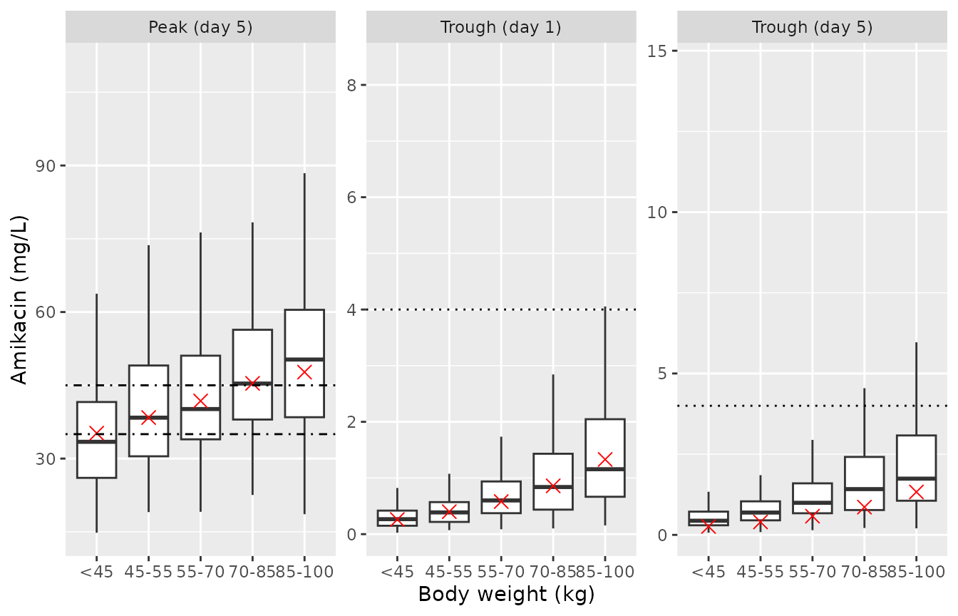
Replicates Figure 4 of Jin 2020: simulated day-5 peak (end of a 1-h infusion) and trough after 12 mg/kg once daily, normal renal function. Dash-dot lines: peak target 35-45 mg/L; dotted line: trough target 4 mg/L. Red crosses: medians digitised from the published figure.
fig4_cmp |>
  transmute(
    wt_group,
    peak_sim = sprintf("%.1f (%.1f-%.1f)", peak_med_sim, peak_q25_sim, peak_q75_sim),
    peak_pub = sprintf("%.1f (%.1f-%.1f)", peak_med_pub, peak_q25_pub, peak_q75_pub),
    trough1_sim = sprintf("%.2f", trough1_med),
    trough5_sim = sprintf("%.2f", trough5_med),
    trough_pub = sprintf("%.2f", trough_med)
  ) |>
  rename(
    "Weight (kg)" = wt_group,
    "Peak, simulated median (IQR)" = peak_sim,
    "Peak, Figure 4 median (IQR)" = peak_pub,
    "Trough day 1, simulated median" = trough1_sim,
    "Trough day 5, simulated median" = trough5_sim,
    "Trough, Figure 4 median" = trough_pub
  ) |>
knitr::kable(caption = "Simulated vs. published (Figure 4) peak and trough, mg/L.")| Weight (kg) | Peak, simulated median (IQR) | Peak, Figure 4 median (IQR) | Trough day 1, simulated median | Trough day 5, simulated median | Trough, Figure 4 median |
|---|---|---|---|---|---|
| <45 | 33.4 (26.1-41.6) | 35.2 (28.0-44.0) | 0.27 | 0.44 | 0.26 |
| 45-55 | 38.4 (30.5-49.1) | 38.4 (30.6-48.6) | 0.39 | 0.69 | 0.40 |
| 55-70 | 40.1 (33.9-51.1) | 41.8 (33.1-52.4) | 0.60 | 0.99 | 0.58 |
| 70-85 | 45.4 (38.0-56.4) | 45.4 (36.0-56.3) | 0.84 | 1.42 | 0.86 |
| 85-100 | 50.3 (38.5-60.5) | 47.7 (38.0-59.8) | 1.16 | 1.74 | 1.33 |
The peaks reproduce Figure 4 in both location (medians within about
5%) and spread. The spread check is what fixes the scale of the printed
residual error: Table 2 prints 0.299 without saying whether
it is a standard deviation or a variance. Read as a variance (SD 0.547),
the log-scale spread of the peaks would be far wider than the published
boxes:
peak_pct <- with(fig4_cmp, 100 * (peak_med_sim / peak_med_pub - 1))
iqr_ratio <- with(fig4_cmp, log(peak_q75_sim / peak_q25_sim) / log(peak_q75_pub / peak_q25_pub))
round(peak_pct, 1)
#> [1] -5.0 -0.1 -4.0 -0.1  5.4
round(iqr_ratio, 2)
#>  75%  75%  75%  75%  75%
#> 1.03 1.03 0.89 0.88 1.00

# Log-scale IQR expected if 0.299 were a variance: the residual SD alone rises
# from 0.299 to 0.547, so the peak log-IQR grows by about 1.7-fold.
sd_other <- sqrt(pmax((with(fig4_cmp, log(peak_q75_pub / peak_q25_pub)) / 1.349)^2 - 0.299^2, 0))
iqr_ratio_if_variance <- sqrt(sd_other^2 + 0.547^2) / sqrt(sd_other^2 + 0.299^2)
round(iqr_ratio_if_variance, 2)
#> [1] 1.69 1.67 1.68 1.71 1.69

stopifnot(
  # Centre: a mis-transcribed V1, weight exponent or dose moves every group by
  # tens of percent.
  abs(median(peak_pct)) < 5,
  max(abs(peak_pct)) < 12,
  # Spread: the SD reading reproduces the published log-IQR (ratio ~1); the
  # variance reading would put it near 1.7.
  abs(median(iqr_ratio) - 1) < 0.2,
  all(iqr_ratio_if_variance > 1.35)
)
The published troughs are first-dose troughs. The day-5 troughs simulated here are 1.3- to 1.7-fold the Figure 4 medians, while the trough 24 h after the first dose reproduces them closely. The difference is accumulation in the slow peripheral compartment (terminal half-life about a day), which the day-5 trough must carry and the figure’s troughs do not. The model is not in question – the same parameters reproduce the figure’s peaks to within a few percent – so the published troughs were most likely read before accumulation, and the day-5 trough is the one this model predicts. Both are kept visible:
tr1_pct <- with(fig4_cmp, 100 * (trough1_med / trough_med - 1))
tr5_ratio <- with(fig4_cmp, trough5_med / trough_med)
round(tr1_pct, 1)
#> [1]   2.5  -3.3   3.5  -2.4 -13.1
round(tr5_ratio, 2)
#> [1] 1.69 1.73 1.71 1.65 1.31
stopifnot(
  abs(median(tr1_pct)) < 15,     # day-1 trough reproduces the published medians
  median(tr5_ratio) > 1.3        # day-5 trough is clearly above them (deviation)
)
Figure 3 and Table 3: target attainment and recommended doses
Figure 3 gives, for each weight group, renal category and once-daily
dose from 7 to 16 mg/kg, the probability that the day-5 peak and trough
fall inside the NTM-PD target (peak 35-45 mg/L, trough < 4 mg/L).
Table 3 reports, for each cell, the dose with the highest probability of
reaching the target. Because the model is linear, the peak and trough at
any dose are the 12 mg/kg values scaled by dose / 12, so
one cohort per cell covers every dose. The simulation classifies a
patient as subtherapeutic if the peak is below 35 mg/L, toxic if the
peak is above 45 mg/L or the trough is 4 mg/L or higher, and therapeutic
otherwise.
subjP <- make_cohort(wt_bands, renal_bands, n_per_arm, 3030)

dosingP <- subjP |>
  tidyr::crossing(time = seq(0, 96, by = 24)) |>
  mutate(evid = 1L, cmt = "central", dur = tinf)
obsP <- subjP |>
  tidyr::crossing(time = c(96 + tinf, 120 - 1e-3)) |>
  mutate(amt = NA_real_, evid = 0L, cmt = "central", dur = NA_real_)
eventsP <- bind_rows(dosingP, obsP) |>
  select(id, time, amt, evid, cmt, dur, WT, CRCL, wt_group, renal) |>
  arrange(id, time, desc(evid))

rxode2::rxSetSeed(3030)
simP <- rxode2::rxSolve(mod, events = eventsP, keep = c("wt_group", "renal")) |>
  as.data.frame()
stopifnot(!anyNA(simP$sim))

pt <- simP |>
  mutate(what = ifelse(time < 100, "peak", "trough")) |>
  select(id, wt_group, renal, what, sim) |>
  tidyr::pivot_wider(names_from = what, values_from = sim)
stopifnot(nrow(pt) == nrow(subjP))

pta <- tidyr::crossing(pt, dose = 7:16) |>
  mutate(
    peak_d = peak * dose / 12, trough_d = trough * dose / 12,
    class = case_when(
      peak_d > 45 | trough_d >= 4 ~ "Toxic",
      peak_d < 35 ~ "Subtherapeutic",
      TRUE ~ "Therapeutic"
    )
  ) |>
  count(wt_group, renal, dose, class) |>
  group_by(wt_group, renal, dose) |>
  mutate(pct = 100 * n / sum(n)) |>
  ungroup() |>
  tidyr::complete(wt_group, renal, dose, class, fill = list(n = 0L, pct = 0))
ggplot(pta, aes(factor(dose), pct, fill = class)) +
  geom_col(position = "dodge") +
  facet_grid(wt_group ~ renal) +
  scale_fill_manual(values = c(Subtherapeutic = "#7fc6e8", Therapeutic = "#2a9d6f",
                               Toxic = "#e0531f")) +
  labs(x = "Dose (mg/kg)", y = "Probability (%)", fill = NULL) +
  theme(legend.position = "bottom")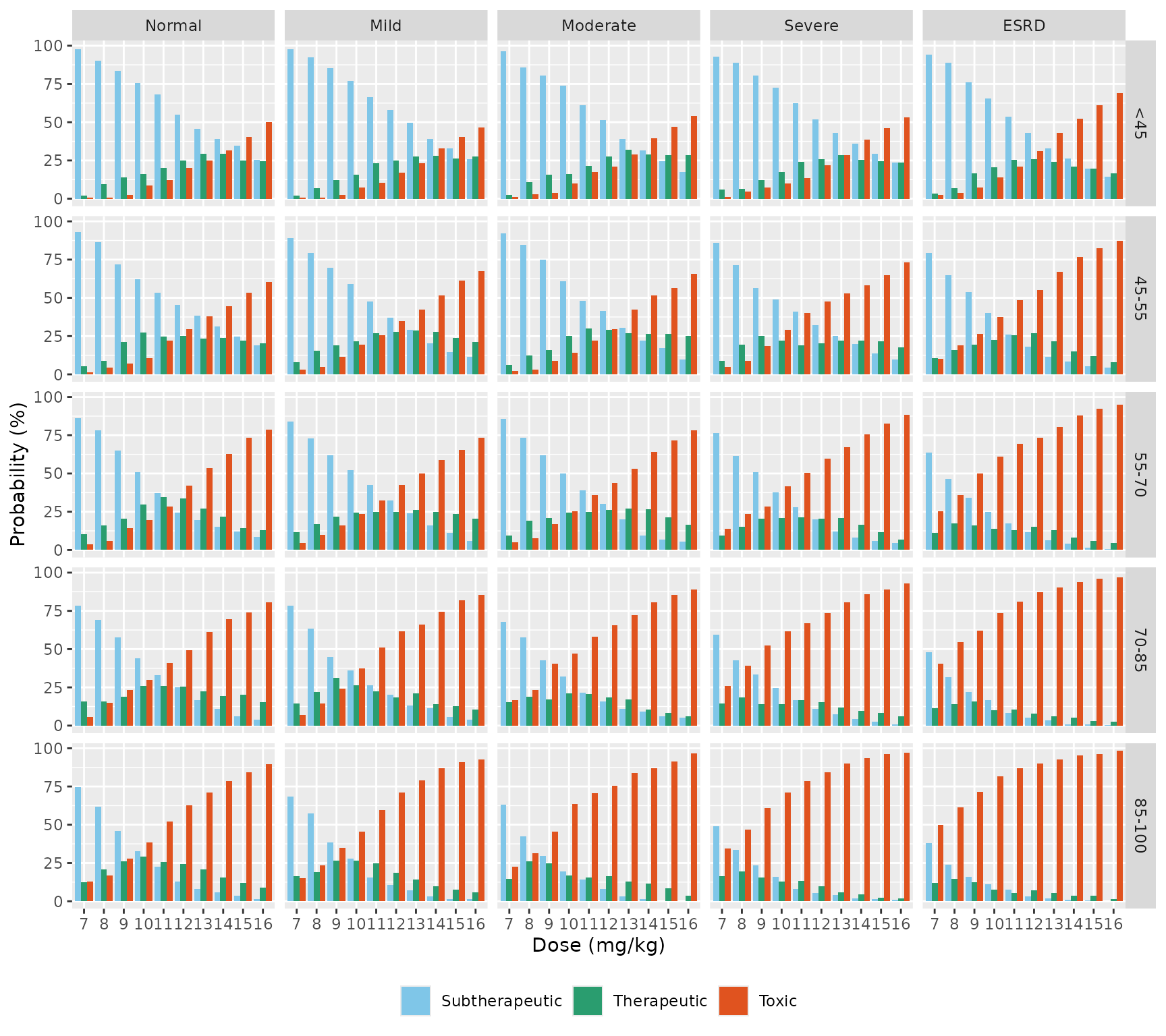
Replicates Figure 3 of Jin 2020: probability of subtherapeutic, therapeutic and toxic day-5 exposure by once-daily dose, renal category (columns) and weight group (rows).
The subtherapeutic and toxic probabilities for the normal-renal-function column at 10, 12 and 14 mg/kg were digitised from Figure 3:
fig3_pub <- tibble::tribble(
  # Digitised by the maintainers from Jin 2020 Figure 3, "Normal" column.
  ~wt_group, ~dose, ~Subtherapeutic, ~Toxic,
  "<45",      10,    70,  10,
  "<45",      12,    50,  23,
  "<45",      14,    31,  39,
  "45-55",    10,    58,  17,
  "45-55",    12,    37,  35,
  "45-55",    14,    22,  53,
  "55-70",    10,    49,  24,
  "55-70",    12,    28,  43,
  "55-70",    14,    15,  61,
  "70-85",    10,    40,  32,
  "70-85",    12,    21,  53,
  "70-85",    14,    10,  71,
  "85-100",   10,    32,  41,
  "85-100",   12,    15,  62,
  "85-100",   14,     7,  78
) |>
  tidyr::pivot_longer(c(Subtherapeutic, Toxic), names_to = "class", values_to = "pct_pub") |>
  mutate(wt_group = factor(wt_group, levels = levels(wt_bands$wt_group)))

fig3_cmp <- pta |>
  filter(renal == "Normal") |>
  select(wt_group, dose, class, pct_sim = pct) |>
  inner_join(fig3_pub, by = c("wt_group", "dose", "class")) |>
  mutate(diff = pct_sim - pct_pub)
stopifnot(nrow(fig3_cmp) == nrow(fig3_pub))

fig3_cmp |>
  mutate(pct_sim = round(pct_sim), diff = round(diff)) |>
  rename("Weight (kg)" = wt_group, "Dose (mg/kg)" = dose, "Class" = class,
         "Simulated (%)" = pct_sim, "Figure 3 (%)" = pct_pub,
         "Difference (points)" = diff) |>
knitr::kable(caption = "Normal renal function: simulated vs. Figure 3 probabilities.")| Weight (kg) | Dose (mg/kg) | Class | Simulated (%) | Figure 3 (%) | Difference (points) |
|---|---|---|---|---|---|
| <45 | 10 | Subtherapeutic | 76 | 70 | 6 |
| <45 | 10 | Toxic | 8 | 10 | -2 |
| <45 | 12 | Subtherapeutic | 55 | 50 | 5 |
| <45 | 12 | Toxic | 20 | 23 | -3 |
| <45 | 14 | Subtherapeutic | 39 | 31 | 8 |
| <45 | 14 | Toxic | 32 | 39 | -8 |
| 45-55 | 10 | Subtherapeutic | 62 | 58 | 4 |
| 45-55 | 10 | Toxic | 10 | 17 | -6 |
| 45-55 | 12 | Subtherapeutic | 46 | 37 | 8 |
| 45-55 | 12 | Toxic | 30 | 35 | -6 |
| 45-55 | 14 | Subtherapeutic | 32 | 22 | 10 |
| 45-55 | 14 | Toxic | 44 | 53 | -8 |
| 55-70 | 10 | Subtherapeutic | 51 | 49 | 2 |
| 55-70 | 10 | Toxic | 20 | 24 | -4 |
| 55-70 | 12 | Subtherapeutic | 24 | 28 | -4 |
| 55-70 | 12 | Toxic | 42 | 43 | -1 |
| 55-70 | 14 | Subtherapeutic | 15 | 15 | 0 |
| 55-70 | 14 | Toxic | 63 | 61 | 2 |
| 70-85 | 10 | Subtherapeutic | 44 | 40 | 4 |
| 70-85 | 10 | Toxic | 30 | 32 | -2 |
| 70-85 | 12 | Subtherapeutic | 25 | 21 | 4 |
| 70-85 | 12 | Toxic | 50 | 53 | -4 |
| 70-85 | 14 | Subtherapeutic | 11 | 10 | 1 |
| 70-85 | 14 | Toxic | 70 | 71 | -2 |
| 85-100 | 10 | Subtherapeutic | 32 | 32 | 0 |
| 85-100 | 10 | Toxic | 38 | 41 | -2 |
| 85-100 | 12 | Subtherapeutic | 13 | 15 | -2 |
| 85-100 | 12 | Toxic | 62 | 62 | 0 |
| 85-100 | 14 | Subtherapeutic | 6 | 7 | -1 |
| 85-100 | 14 | Toxic | 78 | 78 | 0 |
# Proportions of 200 subjects carry a binomial SE of up to 3.5 points, and the
# digitisation adds about 2; a mis-transcribed volume or exponent shifts these by
# 15-30 points.
stopifnot(
  abs(median(fig3_cmp$diff)) < 6,
  median(abs(fig3_cmp$diff)) < 8
)
rec_sim <- pta |>
  filter(class == "Therapeutic") |>
  group_by(wt_group, renal) |>
  slice_max(pct, n = 1, with_ties = FALSE) |>
  ungroup() |>
  select(wt_group, renal, dose_sim = dose)

tab3_pub <- tibble::tribble(
  # Jin 2020 Table 3 (mg/kg once daily).
  ~wt_group, ~Normal, ~Mild, ~Moderate, ~Severe, ~ESRD,
  "<45",      14, 13, 13, 13, 13,
  "45-55",    12, 12, 12, 12, 12,
  "55-70",    11, 11, 11, 11, 10,
  "70-85",    11, 10, 10,  9,  9,
  "85-100",   10, 10, 10,  9,  8
) |>
  tidyr::pivot_longer(-wt_group, names_to = "renal", values_to = "dose_pub") |>
  mutate(wt_group = factor(wt_group, levels = levels(wt_bands$wt_group)),
         renal = factor(renal, levels = levels(renal_bands$renal)))

tab3_cmp <- inner_join(rec_sim, tab3_pub, by = c("wt_group", "renal"))
stopifnot(nrow(tab3_cmp) == 25)

tab3_cmp |>
  mutate(cell = sprintf("%d (%d)", dose_sim, dose_pub)) |>
  select(wt_group, renal, cell) |>
  tidyr::pivot_wider(names_from = renal, values_from = cell) |>
  rename("Weight (kg)" = wt_group) |>
knitr::kable(caption = "Recommended once-daily dose (mg/kg), simulated (Table 3 value in parentheses).")| Weight (kg) | Normal | Mild | Moderate | Severe | ESRD |
|---|---|---|---|---|---|
| <45 | 13 (14) | 14 (13) | 13 (13) | 13 (13) | 12 (13) |
| 45-55 | 10 (12) | 13 (12) | 11 (12) | 9 (12) | 12 (12) |
| 55-70 | 11 (11) | 13 (11) | 13 (11) | 11 (11) | 8 (10) |
| 70-85 | 10 (11) | 9 (10) | 10 (10) | 8 (9) | 9 (9) |
| 85-100 | 10 (10) | 9 (10) | 8 (10) | 8 (9) | 8 (8) |
The therapeutic probability is flat near its maximum (Figure 3 shows adjacent doses within a few points of each other), so the dose that maximises it moves by 1-2 mg/kg between cohorts of this size. The gate is therefore on the pattern of the table – the recommended dose falls with body weight – and on its overall level.
row_mean <- tab3_cmp |>
  group_by(wt_group) |>
  summarise(sim = mean(dose_sim), pub = mean(dose_pub), .groups = "drop")
row_mean
#> # A tibble: 5 × 3
#>   wt_group   sim   pub
#>   <fct>    <dbl> <dbl>
#> 1 <45       13    13.2
#> 2 45-55     11    12
#> 3 55-70     11.2  10.8
#> 4 70-85      9.2   9.8
#> 5 85-100     8.6   9.4
stopifnot(
  row_mean$sim[1] - row_mean$sim[5] > 2,               # published: 13.2 vs 9.4
  abs(mean(tab3_cmp$dose_sim) - mean(tab3_cmp$dose_pub)) < 1.5,
  mean(abs(tab3_cmp$dose_sim - tab3_cmp$dose_pub) <= 2) > 0.7
)
PKNCA validation
NCA is run over the first and fifth dosing intervals of the Figure 4
cohort, separately for each weight group, on the individual predictions
(Cc, no residual error). Over the first interval
Cmin is the pre-dose zero by construction.
nca_in <- sim4 |>
  filter(!is.na(Cc)) |>
  mutate(
    interval = case_when(time <= 24 ~ "Dose 1", time >= 96 & time <= 120 ~ "Dose 5"),
    Cc = pmax(Cc, 0)
  ) |>
  filter(!is.na(interval)) |>
  mutate(
    treatment = paste(interval, wt_group, "kg"),
    time = ifelse(interval == "Dose 5", time - 96, time)
  ) |>
  select(id, treatment, time, Cc)

# Guarantee a time-zero record per subject and interval (the dose-5 interval
# starts on the pre-dose trough, which the grid already contains).
nca_in <- nca_in |>
  distinct(id, treatment, time, .keep_all = TRUE) |>
  arrange(id, treatment, time)
stopifnot(all(tapply(nca_in$time, paste(nca_in$id, nca_in$treatment), min) == 0))

dose_nca <- nca_in |>
  distinct(id, treatment) |>
  left_join(select(subj4, id, amt), by = "id") |>
  mutate(time = 0)

conc_obj <- PKNCA::PKNCAconc(nca_in, Cc ~ time | treatment + id)
dose_obj <- PKNCA::PKNCAdose(dose_nca, amt ~ time | treatment + id)
intervals <- data.frame(start = 0, end = 24, cmax = TRUE, tmax = TRUE,
                        auclast = TRUE, cmin = TRUE)
nca_res <- PKNCA::pk.nca(PKNCA::PKNCAdata(conc_obj, dose_obj, intervals = intervals))

nca_sum <- as.data.frame(nca_res$result) |>
  filter(PPTESTCD %in% c("cmax", "tmax", "auclast", "cmin")) |>
  group_by(treatment, PPTESTCD) |>
  summarise(median = median(PPORRES), .groups = "drop") |>
  tidyr::pivot_wider(names_from = PPTESTCD, values_from = median)

nca_sum |>
  select(treatment, cmax, tmax, auclast, cmin) |>
  rename("Interval / weight group" = treatment, "Cmax (mg/L)" = cmax,
         "Tmax (h)" = tmax, "AUC0-24 (mg*h/L)" = auclast, "Cmin (mg/L)" = cmin) |>
knitr::kable(digits = 2, caption = "Median NCA parameters by dosing interval and weight group.")| Interval / weight group | Cmax (mg/L) | Tmax (h) | AUC0-24 (mg*h/L) | Cmin (mg/L) |
|---|---|---|---|---|
| Dose 1 45-55 kg | 36.50 | 1 | 150.72 | 0.00 |
| Dose 1 55-70 kg | 40.09 | 1 | 195.32 | 0.00 |
| Dose 1 70-85 kg | 43.39 | 1 | 225.56 | 0.00 |
| Dose 1 85-100 kg | 46.01 | 1 | 271.76 | 0.00 |
| Dose 1 <45 kg | 31.31 | 1 | 113.71 | 0.00 |
| Dose 5 45-55 kg | 37.24 | 1 | 160.79 | 0.65 |
| Dose 5 55-70 kg | 41.47 | 1 | 210.88 | 0.99 |
| Dose 5 70-85 kg | 44.89 | 1 | 246.35 | 1.25 |
| Dose 5 85-100 kg | 48.06 | 1 | 299.50 | 1.76 |
| Dose 5 <45 kg | 31.89 | 1 | 120.74 | 0.44 |
At steady state the AUC over a dosing interval equals
Dose / CL for each patient. By day 5 the fast phase is at
steady state and the slow peripheral phase nearly so, so the dose-5
AUC0-24 should sit just below Dose / CL:
cl_i <- sim4 |> distinct(id, cl)
auc5 <- as.data.frame(nca_res$result) |>
  filter(PPTESTCD == "auclast", grepl("^Dose 5", treatment)) |>
  left_join(cl_i, by = "id") |>
  left_join(select(subj4, id, amt), by = "id") |>
  mutate(ratio = PPORRES * cl / amt)
summary(auc5$ratio)
#>    Min. 1st Qu.  Median    Mean 3rd Qu.    Max.
#>  0.9753  0.9935  0.9950  0.9943  0.9960  0.9976
# Deterministic per subject apart from the 15-min trapezoid error; the shortfall
# from 1 is the peripheral accumulation still missing on day 5.
stopifnot(median(auc5$ratio) > 0.95, median(auc5$ratio) < 1.02)
The paper does not report NCA parameters, so there is no published NCA table to compare against; the published exposure summaries it does report (Figures 3 and 4, Table 3) are compared above.
Assumptions and deviations
-
Residual error scale. Table 2 prints the additive
residual error on log-transformed concentrations as
0.299with no scale. It is encoded as a standard deviation (expSd = 0.299, log-normal error on the linear scale) because that reproduces the interquartile ranges of the Figure 4 peaks; read as a variance (SD 0.547), the published boxes would be about 1.7-fold wider on the log scale than they are. -
IIV conversion. Table 2 reports IIV as CV% (CL
27.9%, V1 18%). They are converted with
omega^2 = log(CV^2 + 1); the alternativeomega^2 = CV^2differs by under 4% in the variances and is immaterial. The covariance is used as printed (-0.0135; bootstrap median -0.012), giving a correlation of -0.28. The bootstrap interval printed for the covariance (-0.289 to 0.006) cannot be a covariance interval for these variances (its lower end implies a correlation far below -1) and is presumably a typographic slip for -0.0289; it does not enter the model. - Simulation design not stated. The infusion duration, the time of the peak, and the distributions of weight and eGFR inside each group are not given for the paper’s simulations. A 1-h infusion with the peak at the end of the infusion, and uniform weight and eGFR within each band (normal renal function taken as 90-130 mL/min/1.73 m^2, ESRD as 5-15, lightest weight group from the cohort minimum of 30 kg) are assumed. The Figure 3 classification (toxic = peak above 45 mg/L or trough 4 mg/L or higher) is inferred from the target definition in Methods 4.4.
- Figure 4 troughs. The published troughs are reproduced by the trough 24 h after the first dose, not the day-5 trough, which is 1.3- to 1.7-fold higher because of peripheral accumulation. This is recorded above as a feature of the published simulation; the model parameters are unaffected.
- Supplement. Supplementary Table S1 (sequential covariate model development) confirms the final covariate forms – model 15 combines the power eGFR effect on CL (model 1) with the power weight effect on V1 (model 10), with IIV 27.9% and 18.0% – but prints its OFV as -946.726 against -943.678 in Table 2. The difference is small and does not bear on any parameter value; the Table 2 estimates are used throughout.
-
Covariates screened but not retained (age, height,
serum creatinine, serum albumin, sex) are listed in the model’s
covariatesDataExcluded.