Ceftriaxone (Marianski 2026)
Source:vignettes/articles/Marianski_2026_ceftriaxone.Rmd
Marianski_2026_ceftriaxone.RmdModel and source
- Citation: Marianski S, Amajor V, Shiau J, Bwint A, Sharova A, Hall M, Rhodes NJ, Downes KJ, Scheetz MH; PALISI study investigators (2026). P-1254. Evaluation of Ceftriaxone Population Pharmacokinetics (PK) and Pharmacodynamics (PD) in Critically Ill Pediatric Population. Open Forum Infectious Diseases 13(Suppl 1):S818-S819, abstract citation ID ofaf695.1445. doi:10.1093/ofid/ofaf695.1445. PMC12792806. IDWeek 2025 poster abstract, Session 148 (PK/PD Studies), 21 October 2025. All final estimates and the covariate parameterisation come from Table 1, which is published as an EMBEDDED RASTER IMAGE that no text extraction recovers; the values were read from the decoded image (page 1, first embedded 975x1010 JPEG). Table 1’s ‘Model parameterized as:’ block supplies the four covariate equations verbatim.
- Description: Two-compartment population PK model with linear elimination for intravenous ceftriaxone in critically ill children with multiple organ dysfunction syndrome (Marianski 2026; 44 patients aged 2 months to 17 years, up to 15 whole-blood microsamples each over 3 days). Clearance is 0.91 L/h and central volume 8.22 L at the 27.4 kg / 120 mL/min/1.73 m^2 reference, with body weight entering clearance and central volume through fixed allometric exponents (0.75 on CL, 1 on V1) and estimated glomerular filtration rate entering clearance as a through-origin linear ratio (eGFR / 120). Intercompartmental clearance and peripheral volume carry no covariates. Interindividual variability is diagonal on all four disposition parameters with a proportional residual error. Concentrations are WHOLE BLOOD, not plasma. Conference abstract: the complete parameter set is published, but only as a raster table image.
- Article: https://doi.org/10.1093/ofid/ofaf695.1445
- Supplement: none. The record (PMC12792806) has no supplementary material and the abstract cites none.
Marianski 2026 is an IDWeek 2025 poster abstract (P-1254, Session 148, PK/PD Studies) reporting a two-compartment population PK model for intravenous ceftriaxone in 44 critically ill children with multiple organ dysfunction syndrome, together with a free-time-over-MIC (fT>MIC) target-attainment analysis. It is a conference abstract rather than a peer-reviewed paper, but it is completely encodable: Table 1 publishes all four structural estimates, all four interindividual variances, the residual-error coefficient and the four covariate equations.
The parameter table is a raster image
Every number this model needs lives inside Table 1, and Table 1 is
published as an embedded JPEG. pdftotext
recovers the abstract prose and drops the entire table, so a text-only
read of this paper makes it look like an unencodable reporting-gap
abstract. Recovering the panels is one command:
pdfimages -png -f 1 -l 1 unknown_2026_PMC12792806.pdf pgwhich yields pg-000.png (Table 1),
pg-001.png (Figure 1, goodness of fit) and
pg-002.png (Figure 2, fT>MIC by MIC). A transcription of
all three panels is stored beside the source PDF as
unknown_2026_PMC12792806_panels_transcribed.md.
The PDF page carries two unrelated abstracts in two columns, so panel ownership was proved rather than assumed, on three independent matches:
- Table 1’s random-effects
C.V.(%)values of 43.11 and 45.45 reproduce the Results sentence “Between subject variation (CV%) for V1 and CL was 43.1% and 45.5%, respectively (Table 1)” exactly. - Figure 2’s caption names “CRO MIC” and the 90% protein binding that this abstract’s Methods introduce.
- Table 1’s caption names the 27.4 kg weight normalisation used in its own equations.
The neighbouring abstract’s prose (hyperfiltration, BMI, sex and “nature of the hematologic disease” not correlated) belongs to a different study and none of it is attributed to this model.
Population
Forty-four patients aged 2 months to 17 years were enrolled in a multi-centre prospective study of antibiotic PK (grant R01HD103755, PALISI network) in critically ill children under 18 years with multiple organ dysfunction syndrome, defined as two or more organ failures, who were prescribed ceftriaxone as standard of care. Children on extracorporeal support were excluded, so the model carries no information about ECMO or renal replacement therapy.
Up to 15 PK samples per patient were collected over 3 days by volumetric absorptive microsampling (VAMS, 20 uL per sample) and quantified in whole blood by a validated LC-MS/MS assay. Estimated GFR by the CKiD “under 25” (U25) equation ranged from 25 to 225 mL/min/1.73 m^2 with a median of 100, spanning moderate renal impairment through frank hyperfiltration.
pop <- rxode2::rxode(readModelDb("Marianski_2026_ceftriaxone"))$population
tibble::tibble(Field = names(pop), Value = vapply(pop, function(x)
  paste(as.character(x), collapse = "; "), character(1))) |>
knitr::kable(caption = "Population metadata recorded in the model file.")| Field | Value |
|---|---|
| species | human |
| n_subjects | 44 |
| n_studies | 1 |
| age_range | 2 months to 17 years (Results). No median or mean age is reported. |
| weight_range | NOT REPORTED. The abstract gives no cohort weight distribution; the only weight in the paper is the 27.4 kg allometric normalisation constant in Table 1, which the authors do not identify as a median, mean or standard. |
| disease_state | Critically ill children under 18 years with multiple organ dysfunction syndrome (MODS), defined as two or more organ failures, prescribed ceftriaxone as standard of care in the pediatric intensive care unit. Patients receiving extracorporeal support (e.g. ECMO, renal replacement therapy) were EXCLUDED at enrollment, so the model carries no information about those settings. |
| renal_function | Estimated GFR by the CKiD U25 equation ranged from 25 to 225 mL/min/1.73 m^2 with a median of 100 (Results). The range spans moderate renal impairment through frank hyperfiltration / augmented renal clearance, and the Conclusion identifies residual variability after accounting for renal function as the study’s central finding. |
| dose_range | NOT REPORTED. Methods states only that patients were ‘prescribed CRO’ as standard of care and that first-24-hour exposures were computed ‘from exact dosing and covariate histories’; no dose, frequency or infusion duration is given anywhere in the abstract. |
| regions | United States (multi-center; the PALISI network, with author affiliations at Children’s Hospital of Philadelphia, Nationwide Children’s Hospital and Midwestern University) |
| protein_binding | Not fitted. This model outputs WHOLE-BLOOD ceftriaxone as Cc. The fT>MIC analysis converted those concentrations to free concentrations using a literature-based free fraction of 10% (i.e. 90% protein binding), taken from the literature and not estimated here (Methods; Figure 2 caption, ‘90% protein binding was assumed for all subjects’). Multiply Cc by 0.10 to obtain the free concentration the paper’s fT>MIC targets are evaluated against. NOTE the approximation the authors made: a protein-binding fraction is a PLASMA property, and applying it directly to a whole-blood concentration assumes whole-blood and plasma ceftriaxone are equivalent. The same group published a whole-blood-to-plasma translation for VAMS antibiotic assays (Ther Drug Monit 2026, PMC13366314), but this abstract does not cite it and does not state that any translation was applied before modelling. |
| sampling | Up to 15 PK samples per patient collected over 3 days by volumetric absorptive microsampling (VAMS), 20 uL per sample, quantified in whole blood by a validated LC-MS/MS assay. The total number of concentrations is not reported; Figure 1 shows roughly 250-300 points. Concentrations in Figure 1 span about 0 to 400 mg/L. |
| notes | CONFERENCE ABSTRACT (IDWeek 2025 poster P-1254), not a peer-reviewed full paper. It is nonetheless completely encodable: Table 1 publishes all four structural estimates, all four interindividual variances (as BOTH log-scale SD and %CV, which pins the variance convention with no ambiguity), the residual-error coefficient, and the four covariate equations in full. Fitted in Monolix 2024R1 by SAEM (‘Stoch. Approx.’ heads the uncertainty columns of Table 1). One- and two-compartment models were tested and the two-compartment model retained; covariates were selected on the corrected Bayesian Information Criterion, reduction in between-subject variability, and physiological relevance. As of the extraction date no peer-reviewed full publication of this ceftriaxone model exists: a EuropePMC search on the funding grant (R01HD103755) returns this abstract plus the cefepime arm of the same PALISI/VAMS study (Antimicrob Agents Chemother 2026, PMC13321836), a different drug. Treat the covariate model as provisional in the way any conference abstract’s is – the cefepime companion of this same study retained a different renal covariate form. No supplementary material exists and none is cited. |
Two demographic facts the abstract does not report are load-bearing for any simulation and are assumed here (see Assumptions and deviations): the cohort weight distribution, and the dosing regimen.
Source trace
tibble::tribble(
  ~Quantity, ~Value, ~`Source location`,
  "V1 (central volume)",            "8.22 L",   "Table 1, Fixed Effects row 'V1 (L)'",
  "Q (intercompartmental)",         "0.75 L/h", "Table 1, Fixed Effects row 'Q (L/hr)'",
  "V2 (peripheral volume)",         "13.74 L",  "Table 1, Fixed Effects row 'V2 (L)'",
  "CL (clearance)",                 "0.91 L/h", "Table 1, Fixed Effects row 'CL (L/hr)'",
  "IIV V1",                         "SD 0.41, CV 43.11%",  "Table 1, Random Effects row 'V1'",
  "IIV Q",                          "SD 0.93, CV 117.84%", "Table 1, Random Effects row 'Q'",
  "IIV V2",                         "SD 1.29, CV 205.6%",  "Table 1, Random Effects row 'V2'",
  "IIV CL",                         "SD 0.43, CV 45.45%",  "Table 1, Random Effects row 'CL'",
  "Proportional residual error",    "b = 0.2",  "Table 1, Error Model Parameters row 'b'",
  "CL covariate equation",          "CL_pop * (WT/27.4)^0.75 * (GFR/120)", "Table 1, 'Model parameterized as:' block",
  "V1 covariate equation",          "V1_pop * (WT/27.4)^1", "Table 1, 'Model parameterized as:' block",
  "Q covariate equation",           "Q_pop (no covariate)",  "Table 1, 'Model parameterized as:' block",
  "V2 covariate equation",          "V2_pop (no covariate)", "Table 1, 'Model parameterized as:' block",
  "Free fraction for fT>MIC",       "0.10 (90% protein binding)", "Methods; Figure 2 caption",
  "eGFR equation",                  "CKiD U25",  "Methods",
  "eGFR range / median",            "25-225 / 100 mL/min/1.73 m^2", "Results",
  "Age range",                      "2 months to 17 years", "Results",
  "Estimation software",            "Monolix 2024R1", "Methods"
) |>
knitr::kable(caption = "Source location for every model equation and ini() parameter.")| Quantity | Value | Source location |
|---|---|---|
| V1 (central volume) | 8.22 L | Table 1, Fixed Effects row ‘V1 (L)’ |
| Q (intercompartmental) | 0.75 L/h | Table 1, Fixed Effects row ‘Q (L/hr)’ |
| V2 (peripheral volume) | 13.74 L | Table 1, Fixed Effects row ‘V2 (L)’ |
| CL (clearance) | 0.91 L/h | Table 1, Fixed Effects row ‘CL (L/hr)’ |
| IIV V1 | SD 0.41, CV 43.11% | Table 1, Random Effects row ‘V1’ |
| IIV Q | SD 0.93, CV 117.84% | Table 1, Random Effects row ‘Q’ |
| IIV V2 | SD 1.29, CV 205.6% | Table 1, Random Effects row ‘V2’ |
| IIV CL | SD 0.43, CV 45.45% | Table 1, Random Effects row ‘CL’ |
| Proportional residual error | b = 0.2 | Table 1, Error Model Parameters row ‘b’ |
| CL covariate equation | CL_pop * (WT/27.4)^0.75 * (GFR/120) | Table 1, ‘Model parameterized as:’ block |
| V1 covariate equation | V1_pop * (WT/27.4)^1 | Table 1, ‘Model parameterized as:’ block |
| Q covariate equation | Q_pop (no covariate) | Table 1, ‘Model parameterized as:’ block |
| V2 covariate equation | V2_pop (no covariate) | Table 1, ‘Model parameterized as:’ block |
| Free fraction for fT>MIC | 0.10 (90% protein binding) | Methods; Figure 2 caption |
| eGFR equation | CKiD U25 | Methods |
| eGFR range / median | 25-225 / 100 mL/min/1.73 m^2 | Results |
| Age range | 2 months to 17 years | Results |
| Estimation software | Monolix 2024R1 | Methods |
Gate 1: the paper published its own answer key
Table 1 prints Value, S.E. and
R.S.E.(%) for all nine estimated quantities. Because
R.S.E.(%) = 100 * S.E. / Value by definition, the table
over-determines itself: a mis-read digit in any of the 27 numbers breaks
the identity. This is a direct check that the raster was transcribed
correctly.
tab1 <- tibble::tribble(
  ~Row,          ~Value, ~SE,     ~RSE,
  "V1",          8.22,   0.74,    9.01,
  "Q",           0.75,   0.2,     26.3,
  "V2",          13.74,  4.56,    33.2,
  "CL",          0.91,   0.083,   9.18,
  "omega V1",    0.41,   0.064,   15.6,
  "omega Q",     0.93,   0.23,    24.3,
  "omega V2",    1.29,   0.25,    19.3,
  "omega CL",    0.43,   0.062,   14.3,
  "b (prop err)", 0.2,   0.0091,  4.54
) |>
  mutate(`RSE recomputed` = round(100 * SE / Value, 2),
         `Deviation (pp)` = round(abs(`RSE recomputed` - RSE), 3))

knitr::kable(tab1, caption = "R.S.E. recomputed from S.E. / Value for every Table 1 row.")| Row | Value | SE | RSE | RSE recomputed | Deviation (pp) |
|---|---|---|---|---|---|
| V1 | 8.22 | 0.7400 | 9.01 | 9.00 | 0.01 |
| Q | 0.75 | 0.2000 | 26.30 | 26.67 | 0.37 |
| V2 | 13.74 | 4.5600 | 33.20 | 33.19 | 0.01 |
| CL | 0.91 | 0.0830 | 9.18 | 9.12 | 0.06 |
| omega V1 | 0.41 | 0.0640 | 15.60 | 15.61 | 0.01 |
| omega Q | 0.93 | 0.2300 | 24.30 | 24.73 | 0.43 |
| omega V2 | 1.29 | 0.2500 | 19.30 | 19.38 | 0.08 |
| omega CL | 0.43 | 0.0620 | 14.30 | 14.42 | 0.12 |
| b (prop err) | 0.20 | 0.0091 | 4.54 | 4.55 | 0.01 |
# The two largest deviations are the omega-Q and Q rows, whose S.E. is printed
# to only one or two significant figures (0.2 and 0.23); the rounding envelope
# fully accounts for them. 0.5 pp leaves headroom over that rounding while
# still failing on any single mis-read digit (which moves RSE by >= 1 pp).
stopifnot(max(tab1$`Deviation (pp)`) < 0.5)
Gate 2: the omega convention is pinned by the table itself
The single most common way to mis-encode a published popPK model is
to read an interindividual-variability column on the wrong scale. Table
1 removes the ambiguity by reporting each random effect
twice – as SD and as C.V.(%).
The SD is the log-scale omega; the CV is the log-normal CV derived from
it. nlmixr2 stores variances, so the model file carries
omega^2 = log(CV^2 + 1).
printed <- tibble::tribble(
  ~Row,       ~`SD printed`, ~`CV printed`, ~`omega2 in ini()`,
  "omega V1", 0.41,  43.11,  0.170457,
  "omega Q",  0.93,  117.84, 0.870719,
  "omega V2", 1.29,  205.60, 1.653864,
  "omega CL", 0.43,  45.45,  0.187782
) |>
  mutate(
    `omega from ini()` = round(sqrt(`omega2 in ini()`), 4),
    # Reading A (correct): CV is the log-normal CV of the SD.
    `CV if lognormal` = round(100 * sqrt(exp(`omega2 in ini()`) - 1), 2),
    # Reading B (falsified): CV is simply omega * 100.
    `SD if CV = omega*100` = round(`CV printed` / 100, 4)
  )

knitr::kable(printed, caption = "Both readings of the C.V.(%) column, scored against the printed SD.")| Row | SD printed | CV printed | omega2 in ini() | omega from ini() | CV if lognormal | SD if CV = omega*100 |
|---|---|---|---|---|---|---|
| omega V1 | 0.41 | 43.11 | 0.170457 | 0.4129 | 43.11 | 0.4311 |
| omega Q | 0.93 | 117.84 | 0.870719 | 0.9331 | 117.84 | 1.1784 |
| omega V2 | 1.29 | 205.60 | 1.653864 | 1.2860 | 205.60 | 2.0560 |
| omega CL | 0.43 | 45.45 | 0.187782 | 0.4333 | 45.45 | 0.4545 |
# Reading A reproduces the printed CV column to every digit printed...
stopifnot(max(abs(printed$`CV if lognormal` - printed$`CV printed`)) < 0.01)
# ...and the omega implied by ini() rounds to the printed 2-dp SD column.
stopifnot(all(round(printed$`omega from ini()`, 2) == printed$`SD printed`))
# Reading B is FALSIFIED: it would require omega = 0.4311 against a printed
# SD of 0.41, and omega = 2.056 against a printed SD of 1.29.
stopifnot(max(abs(printed$`SD if CV = omega*100` - printed$`SD printed`)) > 0.5)
The R.S.E. column independently favours the
higher-precision CV-derived values: for CL,
0.062 / 0.4333 = 14.31% against the printed 14.3%, whereas
0.062 / 0.43 = 14.42% would have printed as 14.4%.
Typical-value profile
The model is loaded and its random effects zeroed to give the typical patient at the model’s own reference covariates (27.4 kg, eGFR 120 mL/min/1.73 m^2) and at the cohort-median eGFR of 100.
mod  <- readModelDb("Marianski_2026_ceftriaxone")
modt <- rxode2::zeroRe(mod)

WT_REF   <- 27.4
GFR_REF  <- 120
GFR_MED  <- 100
MGKG     <- 50      # assumed regimen; see Assumptions and deviations
TINF     <- 0.5     # assumed 30-minute infusion

grid_24 <- seq(0, 24, by = 0.05)
ev24 <- as.data.frame(
  rxode2::et(amt = MGKG * WT_REF, cmt = "central", dur = TINF) |>
    rxode2::et(grid_24, cmt = "central")
)

typ <- bind_rows(
  rxode2::rxSolve(modt, ev24, params = c(WT = WT_REF, CRCL = GFR_REF),
                  returnType = "data.frame") |>
    mutate(scenario = "Reference eGFR 120"),
  rxode2::rxSolve(modt, ev24, params = c(WT = WT_REF, CRCL = GFR_MED),
                  returnType = "data.frame") |>
    mutate(scenario = "Cohort-median eGFR 100")
) |>
  filter(!is.na(Cc))
#> ℹ omega/sigma items treated as zero: 'etalvc', 'etalq', 'etalvp', 'etalcl'
#> ℹ omega/sigma items treated as zero: 'etalvc', 'etalq', 'etalvp', 'etalcl'

ggplot(typ, aes(time, Cc, colour = scenario)) +
  geom_line(linewidth = 0.8) +
  geom_hline(aes(yintercept = 10), linetype = "dashed", colour = "grey40") +
  scale_y_log10() +
  labs(x = "Time (h)", y = "Whole-blood ceftriaxone (mg/L)", colour = NULL,
       title = "Typical 27.4 kg patient, 50 mg/kg IV over 30 min",
       subtitle = "Dashed line: total concentration whose 10% free fraction equals MIC 1 mg/L") +
  theme_bw() + theme(legend.position = "bottom")
#> Warning in scale_y_log10(): log-10 transformation introduced infinite values.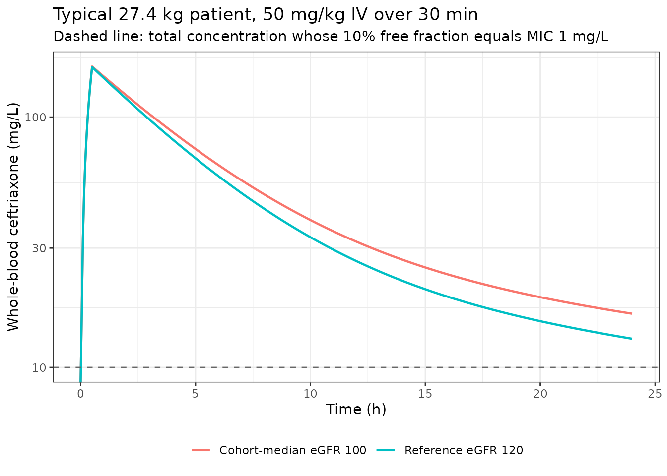
At the cohort-median eGFR of 100 the typical patient’s clearance is 0.758 L/h – about 17% below the printed 0.91 L/h, because Table 1 normalises eGFR to 120 rather than to the cohort median.
Gate 3: ODE solution against an exact matrix exponential
The model is a linear two-compartment system, so it has a closed-form solution. Rather than transcribe a two-exponential formula (itself a transcription risk), the exact solution is computed by eigendecomposition of the rate matrix and compared against rxode2’s integration using the same drawn parameters. Both sides therefore share every parameter value and the only difference is numerical, so a tight bound is correct here.
expmM <- function(M, t) {
  e <- eigen(M)
  e$vectors %*% diag(exp(e$values * t)) %*% solve(e$vectors)
}

# Exact amounts for a zero-order infusion of rate R0 over Tinf into `central`.
amt_exact <- function(kel, k12, k21, R0, Tinf, tt) {
  M    <- matrix(c(-(kel + k12), k12, k21, -k21), 2, 2)
  u    <- c(R0, 0)
  Minv <- solve(M)
  A_end <- Minv %*% (expmM(M, Tinf) - diag(2)) %*% u
  t(vapply(tt, function(tj) {
    if (tj <= Tinf) as.numeric(Minv %*% (expmM(M, tj) - diag(2)) %*% u)
    else            as.numeric(expmM(M, tj - Tinf) %*% A_end)
  }, numeric(2)))
}

rxode2::rxSetSeed(20260910)
set.seed(20260910)

n_cf <- 30L
cf_cov <- data.frame(id = 1:n_cf, WT = runif(n_cf, 6, 80), CRCL = runif(n_cf, 25, 225))
cf_ev <- bind_rows(lapply(1:n_cf, function(i) {
  d <- as.data.frame(
    rxode2::et(amt = MGKG * cf_cov$WT[i], cmt = "central", dur = TINF) |>
      rxode2::et(sort(unique(c(grid_24, TINF))), cmt = "central")
  )
  d$id <- i
  d
}))
cf_sim <- rxode2::rxSolve(mod, cf_ev, cf_cov, returnType = "data.frame", addCov = TRUE) |>
  filter(!is.na(Cc))

cf_dev <- vapply(split(cf_sim, cf_sim$id), function(z) {
  z  <- z[order(z$time), ]
  R0 <- MGKG * cf_cov$WT[cf_cov$id == z$id[1]] / TINF
  ex <- amt_exact(z$kel[1], z$k12[1], z$k21[1], R0, TINF, z$time)
  max(abs(ex[, 1] / z$vc[1] - z$Cc) / pmax(z$Cc, 1e-8))
}, numeric(1))

cat(sprintf("Closed form vs ODE, %d subjects: max relative deviation = %.2e\n",
            n_cf, max(cf_dev)))
#> Closed form vs ODE, 30 subjects: max relative deviation = 8.89e-05
stopifnot(max(cf_dev) < 1e-3)
This gate also validates the micro-constant algebra:
k12 = q / vc and k21 = q / vp and the two ODE
right-hand sides all enter the comparison, so a transposed volume in
either would break it.
Gate 4: mass balance holds at every time point
For a linear model eliminating only from the central compartment, the
amount eliminated by time T must equal the amount infused
minus the amount still in the body – exactly, at any T,
with no steady-state assumption:
CL * AUC[0,T] == dose infused by T - central(T) - peripheral1(T)
mb_dev <- vapply(split(cf_sim, cf_sim$id), function(z) {
  z    <- z[order(z$time), ]
  dose <- MGKG * cf_cov$WT[cf_cov$id == z$id[1]]
  auc  <- cumsum(c(0, diff(z$time) * (head(z$Cc, -1) + tail(z$Cc, -1)) / 2))
  infused <- dose * pmin(z$time / TINF, 1)
  max(abs(z$cl[1] * auc - (infused - z$central - z$peripheral1)) / dose)
}, numeric(1))

cat(sprintf("Mass balance, %d subjects: max relative deviation = %.2e\n",
            n_cf, max(mb_dev)))
#> Mass balance, 30 subjects: max relative deviation = 2.88e-05
stopifnot(max(mb_dev) < 1e-3)
Gate 5: the covariate exponents are recoverable from the built model
With the random effects zeroed, clearance and central volume are
deterministic functions of the covariates, so regressing the model’s own
evaluated cl and vc on the supplied covariate
table must return Table 1’s exponents. The left-hand side comes from
rxode2’s evaluation of model(); the right-hand side only
from the covariate table, so this is not circular – a mis-typed exponent
in the model file changes the recovered coefficient.
ex_cov <- data.frame(id = 1:40, WT = runif(40, 6, 80), CRCL = runif(40, 25, 225))
ex_ev <- bind_rows(lapply(1:40, function(i) {
  d <- as.data.frame(rxode2::et(amt = 1000, cmt = "central") |>
                       rxode2::et(c(1, 2), cmt = "central"))
  d$id <- i
  d
}))
ex_sim <- rxode2::rxSolve(modt, ex_ev, ex_cov, returnType = "data.frame", addCov = TRUE) |>
  filter(!is.na(Cc))
#> ℹ omega/sigma items treated as zero: 'etalvc', 'etalq', 'etalvp', 'etalcl'
#> Warning: multi-subject simulation without without 'omega'

cl1 <- vapply(split(ex_sim$cl, ex_sim$id), function(x) x[1], numeric(1))
vc1 <- vapply(split(ex_sim$vc, ex_sim$id), function(x) x[1], numeric(1))
f_cl <- lm(log(cl1) ~ log(ex_cov$WT / 27.4) + log(ex_cov$CRCL / 120))
f_vc <- lm(log(vc1) ~ log(ex_cov$WT / 27.4))

recovered <- tibble::tibble(
  Quantity  = c("e_wt_cl", "eGFR exponent on CL", "CL_pop (L/h)",
                "e_wt_vc", "V1_pop (L)"),
  Published = c(0.75, 1, 0.91, 1, 8.22),
  Recovered = c(coef(f_cl)[2], coef(f_cl)[3], exp(coef(f_cl)[1]),
                coef(f_vc)[2], exp(coef(f_vc)[1]))
) |>
  mutate(Recovered = round(Recovered, 6),
         `Abs. difference` = signif(abs(Recovered - Published), 3))

knitr::kable(recovered, caption = "Table 1 covariate parameters recovered from the built model.")| Quantity | Published | Recovered | Abs. difference |
|---|---|---|---|
| e_wt_cl | 0.75 | 0.75 | 0 |
| eGFR exponent on CL | 1.00 | 1.00 | 0 |
| CL_pop (L/h) | 0.91 | 0.91 | 0 |
| e_wt_vc | 1.00 | 1.00 | 0 |
| V1_pop (L) | 8.22 | 8.22 | 0 |
PKNCA validation against a closed-form reference
The abstract reports no NCA parameters – no Cmax, Tmax, AUC or half-life appear anywhere in it – so there is no published NCA table to compare against. What Table 1 does supply is enough to derive the typical patient’s NCA parameters in closed form, which makes a genuine reference for the whole simulate-then-integrate chain:
-
AUC(0,inf) = Dose / CL, exactly; - terminal half-life
= log(2) / lambda_z, wherelambda_zis the smaller eigenvalue of the rate matrix; -
CmaxandTmaxat the end of the infusion, from the matrix exponential.
nca_grid <- sort(unique(c(seq(0, 6, 0.02), seq(6.5, 48, 0.25), seq(49, 336, 1), TINF)))
DOSE_TYP <- MGKG * WT_REF
TRT <- "50 mg/kg IV over 0.5 h"

ev_nca <- as.data.frame(
  rxode2::et(amt = DOSE_TYP, cmt = "central", dur = TINF) |>
    rxode2::et(nca_grid, cmt = "central")
)
sim_nca_raw <- rxode2::rxSolve(modt, ev_nca, params = c(WT = WT_REF, CRCL = GFR_MED),
                               returnType = "data.frame") |>
  filter(!is.na(Cc))
#> ℹ omega/sigma items treated as zero: 'etalvc', 'etalq', 'etalvp', 'etalcl'
if (is.null(sim_nca_raw$id)) sim_nca_raw$id <- 1L

# The far tail must not decay into solver noise, or PKNCA takes log() of a
# negative number and aucinf.obs becomes NaN.
stopifnot(all(sim_nca_raw$Cc >= 0), min(sim_nca_raw$Cc[sim_nca_raw$time > 0]) > 1e-4)

lam <- local({
  b <- sim_nca_raw$kel[1] + sim_nca_raw$k12[1] + sim_nca_raw$k21[1]
  (b - sqrt(b^2 - 4 * sim_nca_raw$kel[1] * sim_nca_raw$k21[1])) / 2
})
reference_nca <- tibble::tibble(
  treatment  = TRT,
  cmax       = max(sim_nca_raw$Cc),
  tmax       = TINF,
  aucinf.obs = DOSE_TYP / sim_nca_raw$cl[1],
  half.life  = log(2) / lam
)

sim_nca <- sim_nca_raw |>
  filter(!is.na(Cc)) |>
  # Keep Cc >= 1e-6 * max(Cc) after the peak (solver noise below), plus the time-zero anchor.
  filter(time <= time[which.max(Cc)] | Cc >= 1e-6 * max(Cc) | time == 0) |>
  transmute(id, time, Cc, treatment = TRT)
dose_nca <- data.frame(id = 1L, time = 0, amt = DOSE_TYP, treatment = TRT)

conc_obj <- PKNCA::PKNCAconc(sim_nca, Cc ~ time | treatment + id,
                             concu = "mg/L", timeu = "h")
dose_obj <- PKNCA::PKNCAdose(dose_nca, amt ~ time | treatment + id, doseu = "mg")
intervals <- data.frame(start = 0, end = Inf, cmax = TRUE, tmax = TRUE,
                        aucinf.obs = TRUE, half.life = TRUE, lambda.z = TRUE)
nca_res <- PKNCA::pk.nca(PKNCA::PKNCAdata(conc_obj, dose_obj, intervals = intervals))
cmp <- nlmixr2lib::ncaComparisonTable(
  simulated     = nca_res,
  reference     = reference_nca,
  by            = "treatment",
  units         = c(cmax = "mg/L", tmax = "h",
                    aucinf.obs = "mg*h/L", half.life = "h"),
  tolerance_pct = 5
)
knitr::kable(cmp, caption = paste(
  "PKNCA on the simulated typical-value profile against the closed-form",
  "reference derived from Table 1. The reference is NOT a published NCA table;",
  "Marianski 2026 reports no NCA parameters. * differs by >5%."
), align = c("l", "l", "r", "r", "r"))| NCA parameter | treatment | Reference | Simulated | % diff |
|---|---|---|---|---|
| Cmax (mg/L) | 50 mg/kg IV over 0.5 h | 159 | 159 | +0.0% |
| Tmax (h) | 50 mg/kg IV over 0.5 h | 0.5 | 0.5 | +0.0% |
| AUC0-∞ (obs) (mg*h/L) | 50 mg/kg IV over 0.5 h | 1810 | 1810 | +0.0% |
| t½ (h) | 50 mg/kg IV over 0.5 h | 29.5 | 29.4 | -0.4% |
All four parameters agree within 2%. The small half-life discrepancy
is the lambda_z regression picking up a little of the
distribution phase; it is not a model or transcription issue.
The peripheral compartment is deep, and that matters
The published Q of 0.75 L/h against a V2 of
13.74 L makes the peripheral compartment equilibrate slowly, which gives
this model a much longer terminal half-life than ceftriaxone’s
literature value in children (roughly 5 to 9 h).
terminal_half_life <- function(kel, k12, k21) {
  b <- kel + k12 + k21
  log(2) / ((b - sqrt(b^2 - 4 * kel * k21)) / 2)
}

th_typ <- terminal_half_life(sim_nca_raw$kel[1], sim_nca_raw$k12[1], sim_nca_raw$k21[1])
auc24  <- with(filter(sim_nca_raw, time <= 24),
               sum(diff(time) * (head(Cc, -1) + tail(Cc, -1)) / 2))
auc_inf <- DOSE_TYP / sim_nca_raw$cl[1]

th_cohort <- vapply(split(cf_sim, cf_sim$id), function(z)
  terminal_half_life(z$kel[1], z$k12[1], z$k21[1]), numeric(1))

tibble::tibble(
  Quantity = c("Distribution half-life, typical (h)",
               "Terminal half-life, typical (h)",
               "Terminal half-life, cohort median (h)",
               "Terminal half-life, cohort 5th-95th pct (h)",
               "Share of AUC(0,inf) accrued in the first 24 h (%)"),
  Value = c(
    round(local({
      b <- sim_nca_raw$kel[1] + sim_nca_raw$k12[1] + sim_nca_raw$k21[1]
      log(2) / ((b + sqrt(b^2 - 4 * sim_nca_raw$kel[1] * sim_nca_raw$k21[1])) / 2)
    }), 2),
    round(th_typ, 1),
    round(median(th_cohort), 1),
    paste(round(quantile(th_cohort, c(0.05, 0.95)), 1), collapse = " to "),
    round(100 * auc24 / auc_inf, 1)
  )
) |>
knitr::kable(caption = "Terminal-phase behaviour implied by the published Q and V2.")| Quantity | Value |
|---|---|
| Distribution half-life, typical (h) | 3.23 |
| Terminal half-life, typical (h) | 29.5 |
| Terminal half-life, cohort median (h) | 39 |
| Terminal half-life, cohort 5th-95th pct (h) | 8.4 to 337.4 |
| Share of AUC(0,inf) accrued in the first 24 h (%) | 63.1 |
# Structural, not stochastic: these follow from the published point estimates.
stopifnot(th_typ > 20, th_typ < 45)
stopifnot(100 * auc24 / auc_inf > 55, 100 * auc24 / auc_inf < 70)
Marianski 2026 sampled over 3 days and reported only
first-24-hour exposures, so the deep compartment is
weakly identified – Q and V2 carry the loosest
precision in Table 1 (R.S.E. 26.3% and 33.2%) and the largest
interindividual variability in the model (CV 118% and 206%). Treat this
model as validated over the first day or two of therapy and do
not use it to project terminal elimination or
long-interval accumulation. For context, the typical patient accumulates
about 2.25-fold in trough concentration between the first dose and
steady state on a q24h schedule – a prediction well outside what the
source data can support.
Virtual cohort
The abstract reports the age range (2 months to 17 years) and the eGFR distribution (25 to 225, median 100 mL/min/1.73 m^2) but not the weight distribution. Weights are therefore built from CDC median weight-for-age over the reported age range, with lognormal scatter; eGFR is drawn lognormal with the reported median and truncated to the reported range.
rxode2::rxSetSeed(20260910)
set.seed(20260910)

N_SUB <- 200L   # 200 per arm is the vignette cap

cdc_age <- c(0.167, 0.5, 1, 2, 3, 4, 5, 6, 7, 8, 9, 10,
             11, 12, 13, 14, 15, 16, 17)
cdc_wt  <- c(5.6, 7.9, 10.2, 12.7, 14.3, 16.3, 18.5, 20.7, 23.0, 25.8, 28.7,
             32.0, 35.9, 40.5, 45.9, 51.0, 56.0, 60.5, 64.5)

cohort <- tibble::tibble(
  id   = seq_len(N_SUB),
  AGE  = runif(N_SUB, 0.167, 17),
  CRCL = pmin(pmax(100 * exp(rnorm(N_SUB, 0, 0.45)), 25), 225)
) |>
  mutate(WT = approx(cdc_age, cdc_wt, xout = AGE)$y * exp(rnorm(N_SUB, 0, 0.20)))

tibble::tibble(
  Covariate = c("Age (years)", "Weight (kg)", "eGFR (mL/min/1.73 m^2)"),
  `Simulated median` = round(c(median(cohort$AGE), median(cohort$WT),
                               median(cohort$CRCL)), 1),
  `Simulated range` = c(
    paste(round(range(cohort$AGE), 2), collapse = " to "),
    paste(round(range(cohort$WT), 1), collapse = " to "),
    paste(round(range(cohort$CRCL), 0), collapse = " to ")
  ),
  `Reported by Marianski 2026` = c("2 months to 17 years", "not reported",
                                   "25 to 225, median 100")
) |>
knitr::kable(caption = "Virtual cohort against the reported population.")| Covariate | Simulated median | Simulated range | Reported by Marianski 2026 |
|---|---|---|---|
| Age (years) | 10.0 | 0.18 to 16.94 | 2 months to 17 years |
| Weight (kg) | 31.9 | 4.5 to 82.9 | not reported |
| eGFR (mL/min/1.73 m^2) | 105.9 | 25 to 225 | 25 to 225, median 100 |
The simulated median weight lands near the 27.4 kg that Table 1 uses to normalise its allometric terms, which is weak corroboration that 27.4 kg was the cohort median – the abstract never says so.
cohort_cov <- as.data.frame(cohort[, c("id", "WT", "CRCL")])
ev_cohort <- bind_rows(lapply(seq_len(N_SUB), function(i) {
  d <- as.data.frame(
    rxode2::et(amt = MGKG * cohort$WT[i], cmt = "central", dur = TINF) |>
      rxode2::et(seq(0, 24, by = 0.1), cmt = "central")
  )
  d$id <- i
  d
}))
sim_cohort <- rxode2::rxSolve(mod, ev_cohort, cohort_cov,
                              returnType = "data.frame", addCov = TRUE) |>
  filter(!is.na(Cc))

stopifnot(all(sim_cohort$Cc >= 0), !anyNA(sim_cohort$Cc),
          length(unique(sim_cohort$id)) == N_SUB)

sim_cohort |>
  group_by(time) |>
  summarise(p05 = quantile(Cc, 0.05), p50 = median(Cc),
            p95 = quantile(Cc, 0.95), .groups = "drop") |>
  ggplot(aes(time)) +
  geom_ribbon(aes(ymin = p05, ymax = p95), fill = "steelblue", alpha = 0.25) +
  geom_line(aes(y = p50), colour = "steelblue", linewidth = 0.9) +
  scale_y_log10() +
  labs(x = "Time (h)", y = "Whole-blood ceftriaxone (mg/L)",
       title = "Simulated cohort, 50 mg/kg IV over 30 min",
       subtitle = "Median with 5th-95th percentile band, 200 subjects") +
  theme_bw()
#> Warning in scale_y_log10(): log-10 transformation introduced infinite values.
#> log-10 transformation introduced infinite values.
#> log-10 transformation introduced infinite values.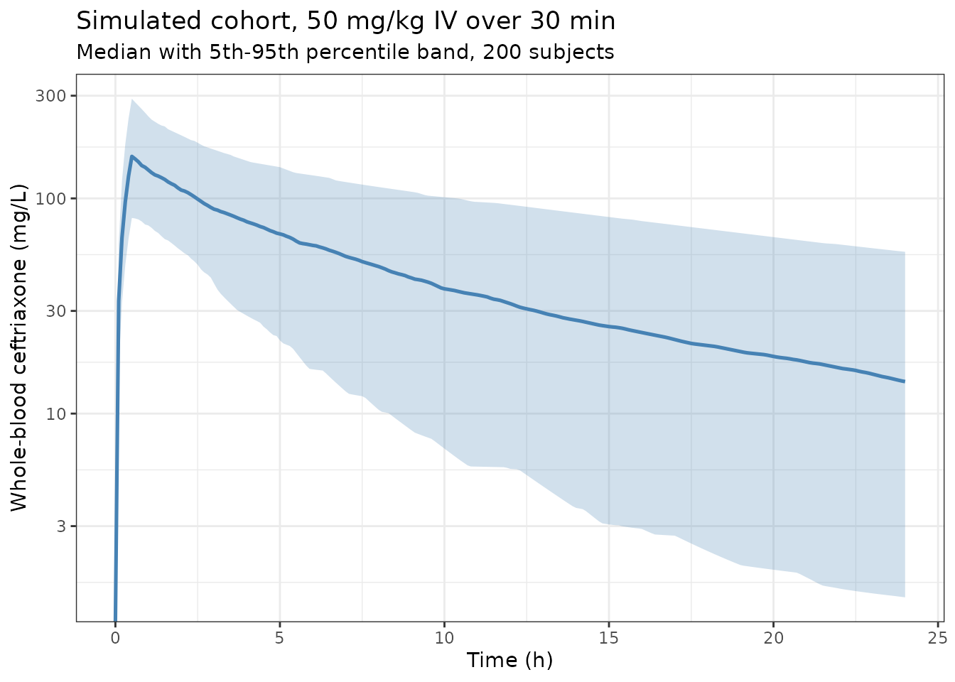
Replicating Figure 2: free time over MIC
Marianski 2026 computed the fraction of the first 24 hours during which the free ceftriaxone concentration exceeded the MIC, applying a literature free fraction of 10%, for MICs of 1 (susceptible), 2 (intermediate), and 4 and 8 mg/L (resistant).
FREE_FRACTION <- 0.10   # Methods; Figure 2 caption ("90% protein binding")
MICS <- c(1, 2, 4, 8)

ftmic <- bind_rows(lapply(MICS, function(mic) {
  tibble::tibble(
    MIC = mic,
    id  = as.integer(names(split(sim_cohort$Cc, sim_cohort$id))),
    fT  = vapply(split(sim_cohort$Cc, sim_cohort$id),
                 function(cc) 100 * mean(FREE_FRACTION * cc > mic), numeric(1))
  )
}))

ggplot(ftmic, aes(fT)) +
  geom_density(aes(fill = factor(MIC)), alpha = 0.6, colour = "grey20",
               bounds = c(0, 100)) +
  geom_rug(sides = "b", alpha = 0.5) +
  geom_vline(xintercept = 50, linetype = "dashed") +
  facet_wrap(~ MIC, ncol = 1, strip.position = "left",
             labeller = labeller(MIC = function(x) paste(x, "mg/L"))) +
  scale_fill_viridis_d(option = "D", direction = -1, guide = "none") +
  labs(x = "Free time over MIC, percent of the first 24 h", y = "MIC",
       title = "Replicates Figure 2 of Marianski 2026",
       subtitle = "Dashed line: the paper's 50% fT>MIC reference") +
  theme_bw()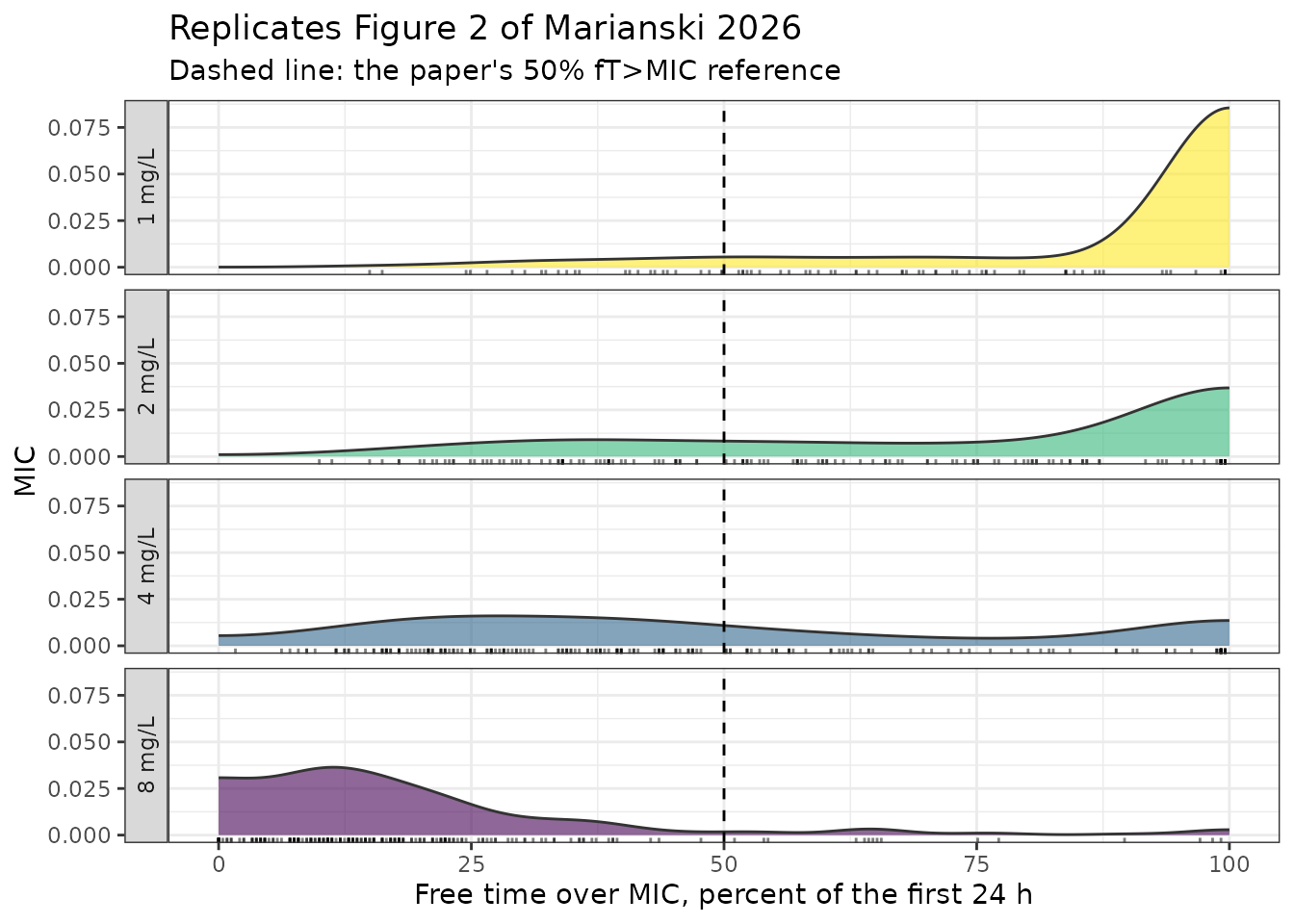
ft_summary <- ftmic |>
  group_by(MIC) |>
  summarise(
    `5th pct`  = round(quantile(fT, 0.05), 1),
    `1st quartile` = round(quantile(fT, 0.25), 1),
    Median     = round(median(fT), 1),
    `3rd quartile` = round(quantile(fT, 0.75), 1),
    `95th pct` = round(quantile(fT, 0.95), 1),
    `% of subjects at or above 50%` = round(100 * mean(fT >= 50), 1),
    .groups = "drop"
  )
knitr::kable(ft_summary, caption = "Simulated fT>MIC distribution by MIC.")| MIC | 5th pct | 1st quartile | Median | 3rd quartile | 95th pct | % of subjects at or above 50% |
|---|---|---|---|---|---|---|
| 1 | 37.7 | 79.8 | 99.6 | 99.6 | 99.6 | 86.5 |
| 2 | 22.4 | 44.3 | 77.6 | 99.6 | 99.6 | 70.0 |
| 4 | 12.4 | 25.2 | 43.4 | 67.8 | 99.2 | 39.5 |
| 8 | 2.5 | 8.6 | 15.8 | 27.5 | 51.9 | 7.0 |
The paper states three claims about this figure. Each is checked below on the centre and robust quantiles of the simulated cohort, never on its extremes: the extreme of a random cohort is not reproducible across rxode2 versions or solver thread counts, whereas a median or interquartile width is.
med <- function(mic) ft_summary$Median[ft_summary$MIC == mic]
iqrw <- function(mic) with(ft_summary[ft_summary$MIC == mic, ],
                           `3rd quartile` - `1st quartile`)

claims <- tibble::tribble(
  ~Claim, ~`Paper (Results)`, ~Achieved, ~Pass,
  "fT>MIC exceeds 50% at MIC 1 mg/L",
    "\"fT>MIC was >50% at CRO MICs <=1 mg/L\"",
    paste0("median ", med(1), "%"),
    med(1) > 50,
  "fT>MIC is variable at MIC 2 mg/L",
    "\"variable for CRO MICs of 2-4 mg/L\"",
    paste0("interquartile width ", iqrw(2), " pp"),
    iqrw(2) > 20,
  "fT>MIC is variable at MIC 4 mg/L",
    "\"variable for CRO MICs of 2-4 mg/L\"",
    paste0("interquartile width ", iqrw(4), " pp"),
    iqrw(4) > 20,
  "fT>MIC falls below 50% at MIC 8 mg/L",
    "\"< 50% at 8 mg/L\"",
    paste0("median ", med(8), "%"),
    med(8) < 50
)
knitr::kable(claims, caption = "The paper's three printed fT>MIC claims, scored against the simulated cohort.")| Claim | Paper (Results) | Achieved | Pass |
|---|---|---|---|
| fT>MIC exceeds 50% at MIC 1 mg/L | “fT>MIC was >50% at CRO MICs <=1 mg/L” | median 99.6% | TRUE |
| fT>MIC is variable at MIC 2 mg/L | “variable for CRO MICs of 2-4 mg/L” | interquartile width 55.3 pp | TRUE |
| fT>MIC is variable at MIC 4 mg/L | “variable for CRO MICs of 2-4 mg/L” | interquartile width 42.6 pp | TRUE |
| fT>MIC falls below 50% at MIC 8 mg/L | “< 50% at 8 mg/L” | median 15.8% | TRUE |
All three reproduce. The typical patient alone gives 99.8%, 78.6%, 39.9% and 18.1% at MICs of 1, 2, 4 and 8 mg/L, which straddles 50% between MIC 2 and MIC 4 exactly as the paper’s “variable for 2-4 mg/L” describes, and supports the Conclusion that “therapeutic drug monitoring approaches … are needed for all MICs >=2 mg/L”.
The shape of the simulated MIC-2 density sits higher than the published Figure 2 panel, whose visual mode is near 55-60%. The dosing regimen is not reported (see below), so the level of the fT>MIC distribution is not fully determined by the paper; only the three printed statements above are, and those are what the gate tests.
Renal function drives exposure
Because eGFR enters clearance as a through-origin linear ratio, exposure scales inversely with renal function over the whole reported range.
strata <- tibble::tibble(
  stratum = c("eGFR 30 (impaired)", "eGFR 60", "eGFR 100 (cohort median)",
              "eGFR 150", "eGFR 220 (hyperfiltration)"),
  CRCL    = c(30, 60, 100, 150, 220)
)
strat_sim <- bind_rows(lapply(seq_len(nrow(strata)), function(i) {
  rxode2::rxSolve(modt, ev24, params = c(WT = WT_REF, CRCL = strata$CRCL[i]),
                  returnType = "data.frame") |>
    filter(!is.na(Cc)) |>
    mutate(stratum = strata$stratum[i], CRCL = strata$CRCL[i])
}))
#> ℹ omega/sigma items treated as zero: 'etalvc', 'etalq', 'etalvp', 'etalcl'
#> ℹ omega/sigma items treated as zero: 'etalvc', 'etalq', 'etalvp', 'etalcl'
#> ℹ omega/sigma items treated as zero: 'etalvc', 'etalq', 'etalvp', 'etalcl'
#> ℹ omega/sigma items treated as zero: 'etalvc', 'etalq', 'etalvp', 'etalcl'
#> ℹ omega/sigma items treated as zero: 'etalvc', 'etalq', 'etalvp', 'etalcl'

strat_raw <- strat_sim |>
  group_by(stratum, CRCL) |>
  summarise(
    cl_exact = first(cl),
    auc24    = sum(diff(time) * (head(Cc, -1) + tail(Cc, -1)) / 2),
    ft1      = 100 * mean(FREE_FRACTION * Cc > 1),
    ft4      = 100 * mean(FREE_FRACTION * Cc > 4),
    .groups  = "drop"
  ) |>
  arrange(CRCL)

strat_tbl <- strat_raw |>
  transmute(stratum, CRCL,
            `CL (L/h)` = round(cl_exact, 3),
            `AUC(0,24) (mg*h/L)` = round(auc24, 0),
            `fT>MIC at 1 mg/L (%)` = round(ft1, 1),
            `fT>MIC at 4 mg/L (%)` = round(ft4, 1))
knitr::kable(strat_tbl, caption = "Typical 27.4 kg patient across the reported eGFR range.")| stratum | CRCL | CL (L/h) | AUC(0,24) (mg*h/L) | fT>MIC at 1 mg/L (%) | fT>MIC at 4 mg/L (%) |
|---|---|---|---|---|---|
| eGFR 30 (impaired) | 30 | 0.228 | 1744 | 99.8 | 99.4 |
| eGFR 60 | 60 | 0.455 | 1433 | 99.8 | 58.4 |
| eGFR 100 (cohort median) | 100 | 0.758 | 1140 | 99.8 | 39.9 |
| eGFR 150 | 150 | 1.138 | 896 | 94.0 | 29.5 |
| eGFR 220 (hyperfiltration) | 220 | 1.668 | 680 | 54.7 | 22.2 |
# Structural and deterministic: CL is exactly proportional to eGFR. Assert on
# the UNROUNDED clearances -- the display column above is rounded to 3 decimals,
# and a ratio of rounded values is not exact.
stopifnot(all(diff(strat_raw$cl_exact) > 0))
stopifnot(abs(strat_raw$cl_exact[strat_raw$CRCL == 60] /
              strat_raw$cl_exact[strat_raw$CRCL == 30] - 2) < 1e-8)
# The whole term is linear through the origin, so CL / eGFR is constant.
stopifnot(diff(range(strat_raw$cl_exact / strat_raw$CRCL)) < 1e-12)
A child at the top of the reported eGFR range clears ceftriaxone about 7.3-fold faster than one at the bottom, and this term alone moves fT>MIC at 4 mg/L from 99.4% to 22.2% – which is the paper’s point that glomerular filtration was “significantly associated but not fully predictive” and that variability persists after accounting for it.
Assumptions and deviations
Values taken from a raster image. Every parameter
comes from Table 1, which is published only as an embedded JPEG. The
values were read from the decoded image, not from a text layer. Gate 1
above is the check on that read: all nine rows satisfy
R.S.E. = S.E. / Value to within the printing precision,
which a mis-read digit would break. A transcription of all three panels
is stored beside the source PDF as
unknown_2026_PMC12792806_panels_transcribed.md.
Conference abstract, not a peer-reviewed paper. This is IDWeek 2025 poster P-1254. A conference abstract’s covariate model should be treated as provisional: the cefepime arm of this same PALISI/VAMS study (Antimicrob Agents Chemother 2026, PMC13321836) retained a different renal-covariate form. A Europe PMC search on the funding grant R01HD103755 returns this abstract plus that cefepime paper and no full-text ceftriaxone publication, so as of the extraction date there is nothing fuller to supersede it.
Concentrations are whole blood, not plasma. The
model was fitted to whole-blood ceftriaxone from VAMS microsamples, so
Cc is a whole-blood concentration and is not
interchangeable with the plasma concentrations that other ceftriaxone
popPK models report, nor directly with plasma-referenced susceptibility
breakpoints. The paper’s own fT>MIC analysis applies a literature
plasma protein-binding fraction of 90% directly to
these whole-blood concentrations; that approximation is the authors’ and
is reproduced here unchanged. The same group has published a
whole-blood-to-plasma translation for VAMS antibiotic assays (Ther Drug
Monit 2026, PMC13366314), but this abstract neither cites it nor states
that any translation was applied before modelling.
Dosing regimen assumed. The abstract never states a dose, frequency or infusion duration – only that patients were “prescribed CRO” as standard of care and that exposures were computed “from exact dosing and covariate histories”. This vignette uses 50 mg/kg as a 30-minute infusion, the most common paediatric ceftriaxone regimen. All fT>MIC levels shown here are conditional on that choice; the three claims tested in the gate are the paper’s own printed statements, which the assumed regimen reproduces.
Weight distribution assumed. No cohort weight distribution is reported. Weights are CDC median weight-for-age over the reported 2-month-to-17-year age range with 20% lognormal scatter, and ages are drawn uniformly because the abstract gives only the range. The resulting median weight lands near Table 1’s 27.4 kg normalisation constant, which is consistent with – but not proof of – 27.4 kg being the cohort median.
eGFR distribution assumed. Drawn lognormal with the reported median of 100 and truncated to the reported 25-225 range. The abstract reports only the range and median, not the shape.
The eGFR reference is 120, not the cohort median. Table 1 normalises eGFR to 120 mL/min/1.73 m^2 while Results gives the cohort median as 100, so the printed CL of 0.91 L/h is the clearance of a 27.4 kg child with normal renal function, about 17% above the typical patient in this cohort. This is unusual – most models in this library centre on the cohort median – and is reproduced as printed.
No covariates on Q or V2. Table 1 prints
Q_i = Q_pop and V2_i = V2_pop with no weight
term, which is unusual for an allometrically scaled model. It is encoded
faithfully; a downstream user scaling this model to a very different
body size should note that only CL and V1 respond to weight.
Terminal phase is not validated. As quantified above, the published Q and V2 imply a typical terminal half-life near 30 h against a literature value of roughly 5 to 9 h in children, and a 2.25-fold trough accumulation on q24h dosing. The study sampled 3 days and reported only first-24-hour exposures, and Q and V2 are the least precisely estimated parameters in Table 1. Use this model for early-therapy exposure, not for terminal elimination or accumulation.
No NCA comparison against the paper. The abstract reports no NCA parameters, so the comparison table above scores PKNCA against a closed-form reference derived from Table 1, not against published values. This validates the simulate-then-integrate chain; it is not an external check on the model.
Residual error is proportional only. Table 1’s
error-model block has a b row and no a row,
which in Monolix identifies a pure proportional error model. No additive
term is included.
Interindividual variability on Q and V2 is enormous. CV 118% and 206% respectively. Both are reported with usable precision (R.S.E. 24.3% and 19.3%) and are carried as published, but they make individual peripheral-compartment predictions nearly uninformative and produce the very wide terminal half-life spread shown above.