Voriconazole (Khan-asa 2020)
Source:vignettes/articles/KhanAsa_2020_voriconazole.Rmd
KhanAsa_2020_voriconazole.RmdModel and source
- Citation: Khan-asa B, Punyawudho B, Singkham N, Chaivichacharn P, Karoopongse E, Montakantikul P, Chayakulkeeree M. Impact of Albumin and Omeprazole on Steady-State Population Pharmacokinetics of Voriconazole and Development of a Voriconazole Dosing Optimization Model in Thai Patients with Hematologic Diseases. Antibiotics (Basel). 2020;9(9):574. doi:10.3390/antibiotics9090574
- Description: One-compartment population pharmacokinetic model with first-order absorption and linear elimination for oral voriconazole at steady state in Thai adults with hematologic diseases (Khan-asa 2020); apparent clearance falls linearly with serum albumin below 3.2 g/dL and by 30.6% with concomitant omeprazole 40 mg/day or more, and the absorption rate constant is fixed at 1.1 per hour
- Article (open access): https://doi.org/10.3390/antibiotics9090574
mod <- readModelDb("KhanAsa_2020_voriconazole")
ui <- rxode2::rxode(mod)
#> ℹ parameter labels from comments will be replaced by 'label()'
Population
Khan-asa and colleagues report the first population pharmacokinetic analysis of voriconazole in Thai adults with hematologic diseases. Sixty-five patients at Siriraj Hospital, Bangkok, took oral voriconazole for prophylaxis or treatment of invasive aspergillosis: a loading dose of 400 mg every 12 h (two doses), then 200 mg every 12 h. All 237 plasma concentrations were drawn at steady state - 126 from 18 patients sampled intensively on day 7 (0, 1, 1.5, 2, 4, 8 and 12 h) and 111 trough-type samples from 47 patients between day 7 and day 40. The median observed concentration was 4.49 mg/L.
Table 1 of the paper summarises the cohort: 63% male, mean age 47.7 years (20-78), mean weight 58.6 kg (27.2-105), acute myeloid leukaemia in 57%. Mean serum albumin was 3.04 g/dL (1.60-4.3; median 3.2 g/dL), so the typical patient was hypoalbuminaemic. Omeprazole was very common: 20 mg/day in 44.6% and 40 mg/day in 26.2% of patients. CYP2C19 genotype (1 ultra-rapid, 33 extensive, 24 intermediate, 7 poor metabolizers) was screened but not retained.
The final model is one-compartment with first-order absorption (Ka fixed at 1.1 /h) and linear elimination; apparent clearance falls linearly with albumin below the median and is 30.6% lower in patients taking omeprazole 40 mg/day or more. Only clearance carries between-subject variability, and the residual error is additive.
The same information is available programmatically via
readModelDb("KhanAsa_2020_voriconazole")()$population.
Source trace
| Equation / parameter | Value | Source location |
|---|---|---|
| One-compartment, first-order absorption and elimination | n/a | Section 2.2; Supplementary S1 (ADVAN2 TRANS2) |
lka (Ka, fixed) |
1.1 /h | Table 2, row Ka (/h) = FIX 1.100; Section
2.2 (fixed from Pascual 2012) |
lcl (CL/F) |
3.43 L/h | Table 2, row CL/F (L/h)
|
lvc (V/F) |
47.6 L | Table 2, row V/F (L)
|
e_alb_cl |
0.249 per g/dL | Table 2, row CL-albumin
|
e_ome40_cl |
-0.306 | Table 2, row CL-omeprazole >= 40 mg/day
|
etalcl |
0.226 (50.4% CV) | Table 2, row IIV-CL
|
addSd |
sqrt(2.67) = 1.634 mg/L | Table 2, row RUV (mg/L) = 2.67, read as a variance (see
below) |
CL/F = 3.43 x [1 + 0.249 x (ALB - 3.2)] x [1 + (-0.306 x OME)] |
n/a | Section 2.2, final-model equation |
| Albumin centring value 3.2 g/dL | n/a | Section 2.4 (median albumin 3.2 g/dL); Section 4.5 (centred on median) |
OME = 1 for omeprazole >= 40 mg/day, 0 for <= 20
mg/day |
n/a | Section 2.2, text below the equation |
| Additive residual error | n/a | Section 2.2 (“described using an additive model”) |
Two unit notes. The package’s canonical albumin column
ALB is in g/L, so the model multiplies it by 0.1 before
applying the paper’s per-g/dL slope. The paper’s omeprazole indicator is
supplied as the daily omeprazole dose, DOSE_OMEPRAZOLE_MGD,
and the model sets the indicator to 1 when that dose is 40 mg/day or
more. A plain yes/no omeprazole column would be wrong here, because the
paper tested omeprazole 20 mg/day and did not retain it.
Structural gates
Deterministic checks on the typical-value model, run before any cohort is drawn.
tau <- 12
ndose <- 20L # 240 h; the slowest typical half-life below is about 17 h
t_start <- (ndose - 1L) * tau

typical_profile <- function(alb_gL, ome_mgd, dose = 200) {
  ev <- rxode2::et(amt = dose, ii = tau, addl = ndose - 1L, cmt = "depot") |>
    rxode2::et(seq(t_start, t_start + tau, by = 0.1), cmt = "central")
  d <- as.data.frame(ev)
  d$id <- 1L
  d$ALB <- alb_gL
  d$DOSE_OMEPRAZOLE_MGD <- ome_mgd
  rxode2::rxSolve(rxode2::zeroRe(mod), d, returnType = "data.frame", addDosing = FALSE)
}

ref <- typical_profile(alb_gL = 32, ome_mgd = 0)
#> ℹ parameter labels from comments will be replaced by 'label()'
#> ℹ omega/sigma items treated as zero: 'etalcl'
Gate 1 - every declared ODE state survives the
solve. A model defining cl and vc can
be silently matched against rxode2’s analytic kernel, discarding the
explicit d/dt() bodies.
Gate 2 - the covariate equation. At the median albumin (3.2 g/dL = 32 g/L) and without omeprazole 40 mg/day, clearance must equal the printed typical value; each covariate must move it by exactly the printed factor. Omeprazole 20 mg/day must have no effect.
cl_at <- function(alb_gL, ome_mgd) typical_profile(alb_gL, ome_mgd)$cl[1]
cl_tbl <- tibble::tibble(
  scenario = c("ALB 3.2 g/dL, no omeprazole", "ALB 3.2 g/dL, omeprazole 20 mg/day",
               "ALB 3.2 g/dL, omeprazole 40 mg/day", "ALB 2.0 g/dL, no omeprazole",
               "ALB 4.2 g/dL, omeprazole 40 mg/day"),
  alb = c(32, 32, 32, 20, 42), ome = c(0, 20, 40, 0, 40)
) |>
  dplyr::rowwise() |>
  dplyr::mutate(
    cl_model = cl_at(alb, ome),
    cl_paper = 3.43 * (1 + 0.249 * (alb / 10 - 3.2)) * (1 - 0.306 * (ome >= 40))
  ) |>
  dplyr::ungroup()
#> ℹ parameter labels from comments will be replaced by 'label()'
#> ℹ omega/sigma items treated as zero: 'etalcl'
#> ℹ parameter labels from comments will be replaced by 'label()'
#> ℹ omega/sigma items treated as zero: 'etalcl'
#> ℹ parameter labels from comments will be replaced by 'label()'
#> ℹ omega/sigma items treated as zero: 'etalcl'
#> ℹ parameter labels from comments will be replaced by 'label()'
#> ℹ omega/sigma items treated as zero: 'etalcl'
#> ℹ parameter labels from comments will be replaced by 'label()'
#> ℹ omega/sigma items treated as zero: 'etalcl'

knitr::kable(
  cl_tbl |>
    dplyr::select(scenario, cl_model, cl_paper) |>
    dplyr::rename("Scenario" = scenario, "Model CL/F (L/h)" = cl_model,
                  "Section 2.2 equation (L/h)" = cl_paper),
  digits = 3
)| Scenario | Model CL/F (L/h) | Section 2.2 equation (L/h) |
|---|---|---|
| ALB 3.2 g/dL, no omeprazole | 3.430 | 3.430 |
| ALB 3.2 g/dL, omeprazole 20 mg/day | 3.430 | 3.430 |
| ALB 3.2 g/dL, omeprazole 40 mg/day | 2.380 | 2.380 |
| ALB 2.0 g/dL, no omeprazole | 2.405 | 2.405 |
| ALB 4.2 g/dL, omeprazole 40 mg/day | 2.973 | 2.973 |
Gate 3 - steady-state mass balance. Over one dosing
interval at steady state, CL/F x AUCtau = Dose. Both sides
use the same parameters, so the only error is numerical and a tight
bound is correct.
auc_tau <- PKNCA::pk.calc.auc(
  conc = ref$Cc, time = ref$time,
  interval = c(t_start, t_start + tau), method = "linear"
)
mass_ratio <- ref$cl[1] * auc_tau / 200
cat(sprintf("CL/F = %.3f L/h; AUCtau = %.2f mg*h/L; CL*AUCtau/Dose = %.4f\n",
            ref$cl[1], auc_tau, mass_ratio))
#> CL/F = 3.430 L/h; AUCtau = 58.31 mg*h/L; CL*AUCtau/Dose = 0.9999
stopifnot(abs(mass_ratio - 1) < 0.005)
Residual error: variance, not standard deviation
Table 2 prints RUV (mg/L) = 2.67. The same table prints
between-subject variability of clearance as the variance 0.226 (with
(%CV) 50.40%, since sqrt(exp(0.226) - 1) = 0.504), so the
table is raw NONMEM $OMEGA / $SIGMA output and
2.67 is most naturally the additive variance. The model
carries its square root, 1.634 mg/L.
The traditional VPC in Supplementary Figure S1 confirms it. Its simulated 5th-percentile band is centred near 2.7 mg/L at 1.5 h after the dose, about 2 mg/L at 5 h and about 0 at 12 h. Only an additive SD of 1.63 mg/L puts the 5th percentile there; an SD of 2.67 mg/L puts it at or below the lower edge of the band. The comparison below uses a deterministic quadrature grid, not random draws, so it is identical on every machine.
cmin_ss <- function(cl, t, dose = 200, v = 47.6, ka = 1.1) {
  k <- cl / v
  dose * ka / (v * (ka - k)) *
    (exp(-k * t) / (1 - exp(-k * tau)) - exp(-ka * t) / (1 - exp(-ka * tau)))
}
# Quadrature over the albumin distribution (Table 1: mean 3.04, SD 0.61
# g/dL), the omeprazole 40 mg/day fraction (26%) and the clearance eta.
grid <- tidyr::expand_grid(
  alb = qnorm((1:25 - 0.5) / 25, 3.04, 0.61),
  ome = c(0, 1),
  z = qnorm((1:200 - 0.5) / 200)
) |>
  dplyr::mutate(
    w = ifelse(ome == 1, 0.26, 0.74),
    cl = 3.43 * (1 + 0.249 * (pmin(pmax(alb, 1.6), 4.3) - 3.2)) *
      (1 - 0.306 * ome) * exp(z * sqrt(0.226))
  )
p05_at <- function(t, sd) {
  mu <- cmin_ss(grid$cl, t)
  f <- function(q) sum(grid$w * pnorm(q, mu, sd)) / sum(grid$w) - 0.05
  uniroot(f, c(-20, 20))$root
}
ruv_tbl <- tidyr::expand_grid(t = c(1.5, 5, 12), sd = c(sqrt(2.67), 2.67)) |>
  dplyr::rowwise() |>
  dplyr::mutate(p05 = p05_at(t, sd)) |>
  dplyr::ungroup() |>
  dplyr::mutate(fig_s1 = c(2.7, 2.7, 2, 2, 0, 0))
knitr::kable(
  ruv_tbl |>
    dplyr::rename("Time after dose (h)" = t, "Additive SD (mg/L)" = sd,
                  "Model 5th percentile (mg/L)" = p05,
                  "Figure S1 band centre (mg/L, read by eye)" = fig_s1),
  digits = 2
)| Time after dose (h) | Additive SD (mg/L) | Model 5th percentile (mg/L) | Figure S1 band centre (mg/L, read by eye) |
|---|---|---|---|
| 1.5 | 1.63 | 2.68 | 2.7 |
| 1.5 | 2.67 | 1.43 | 2.7 |
| 5.0 | 1.63 | 1.79 | 2.0 |
| 5.0 | 2.67 | 0.57 | 2.0 |
| 12.0 | 1.63 | -0.10 | 0.0 |
| 12.0 | 2.67 | -1.37 | 0.0 |
Replicating the dosing simulation (Figures 3 and 4)
The paper simulated steady-state troughs for 50-400 mg every 12 h, stratified by albumin band and omeprazole group, and reported the percentage in the therapeutic (1-5 mg/L), toxic (> 5 mg/L) and sub-therapeutic (< 1 mg/L) ranges. The text quotes one cell in full: albumin 1.5-2 g/dL at 150 mg every 12 h. The percentages it quotes are multiples of 1/138 and 1/140, so each cell rests on only about 140 simulated patients and carries a binomial standard error of roughly 4 percentage points.
The replication below computes those percentages exactly by quadrature over the clearance eta and a uniform albumin distribution within each band. The paper’s troughs carry no residual error (adding it would put about 8% of the low-albumin 150 mg group below 1 mg/L; the paper reports 2.9%), so none is added here.
band_pct <- function(dose, alb_lo, alb_hi, ome) {
  g <- tidyr::expand_grid(
    alb = seq(alb_lo, alb_hi, length.out = 21),
    z = qnorm((1:2000 - 0.5) / 2000)
  )
  cl <- 3.43 * (1 + 0.249 * (g$alb - 3.2)) * (1 - 0.306 * ome) * exp(g$z * sqrt(0.226))
  c0 <- cmin_ss(cl, tau, dose = dose)
  c(sub = 100 * mean(c0 < 1), ther = 100 * mean(c0 >= 1 & c0 <= 5),
    tox = 100 * mean(c0 > 5))
}
ex <- tibble::tibble(
  group = c("No omeprazole / 20 mg/day", "Omeprazole 40 mg/day"),
  ome = c(0, 1),
  paper_ther = c(51.45, 22.86), paper_tox = c(45.65, 76.43), paper_sub = c(2.90, 0.71)
) |>
  dplyr::rowwise() |>
  dplyr::mutate(
    p = list(band_pct(150, 1.5, 2.0, ome)),
    model_ther = p[["ther"]], model_tox = p[["tox"]], model_sub = p[["sub"]]
  ) |>
  dplyr::ungroup() |>
  dplyr::select(-p, -ome)

knitr::kable(
  ex |>
    dplyr::rename("Group (albumin 1.5-2 g/dL, 150 mg q12h)" = group,
                  "Paper % 1-5 mg/L" = paper_ther, "Model % 1-5 mg/L" = model_ther,
                  "Paper % > 5 mg/L" = paper_tox, "Model % > 5 mg/L" = model_tox,
                  "Paper % < 1 mg/L" = paper_sub, "Model % < 1 mg/L" = model_sub),
  digits = 1,
  caption = "Section 2.4 worked example against the model (deterministic)."
)| Group (albumin 1.5-2 g/dL, 150 mg q12h) | Paper % 1-5 mg/L | Paper % > 5 mg/L | Paper % < 1 mg/L | Model % 1-5 mg/L | Model % > 5 mg/L | Model % < 1 mg/L |
|---|---|---|---|---|---|---|
| No omeprazole / 20 mg/day | 51.5 | 45.6 | 2.9 | 55.7 | 42.5 | 1.7 |
| Omeprazole 40 mg/day | 22.9 | 76.4 | 0.7 | 28.1 | 71.7 | 0.2 |
# Within about 1.5 binomial standard errors of the paper's ~140-patient cells.
stopifnot(all(abs(ex$model_ther - ex$paper_ther) < 7))
stopifnot(all(abs(ex$model_tox - ex$paper_tox) < 7))
# Omeprazole 40 mg/day raises exposure, so it shifts patients toxic.
stopifnot(ex$model_tox[2] > ex$model_tox[1])
The full grid is shown below for all four albumin bands in the no-omeprazole group. In the lowest band the model and Figure 3 agree throughout; in the higher bands Figure 3 is much flatter across albumin than the printed covariate equation implies. At 50 mg every 12 h and albumin 4.01-4.5 g/dL, for instance, typical CL/F from the Section 2.2 equation is about 4.3 L/h and the typical steady-state trough about 0.8 mg/L, so most patients should fall below 1 mg/L. Figure 3 instead shows 32% below 1 mg/L and 66% in range. The figure cannot be reproduced from the published parameters at those bands. The model follows the printed equation and Table 2 and was not adjusted to match the figure.
doses <- c(50, 100, 150, 200, 250, 300, 350, 400)
bands <- tibble::tibble(
  band = c("Alb 1.5-2.00 g/dL", "Alb 2.01-3.00 g/dL", "Alb 3.01-4.00 g/dL", "Alb 4.01-4.5 g/dL"),
  lo = c(1.5, 2.01, 3.01, 4.01), hi = c(2.0, 3.0, 4.0, 4.5)
)
fig3 <- tidyr::expand_grid(bands, dose = doses) |>
  dplyr::rowwise() |>
  dplyr::mutate(p = list(band_pct(dose, lo, hi, 0))) |>
  dplyr::ungroup() |>
  tidyr::unnest_wider(p) |>
  tidyr::pivot_longer(c(sub, ther, tox), names_to = "range", values_to = "pct") |>
  dplyr::mutate(range = dplyr::recode(range, sub = "< 1 mg/L", ther = "1-5 mg/L", tox = "> 5 mg/L"))

ggplot(fig3, aes(dose, pct, colour = range)) +
  geom_line() + geom_point() +
  facet_wrap(~band) +
  labs(x = "Voriconazole maintenance dose every 12 h (mg)", y = "Percentage (%)", colour = NULL) +
  theme_bw()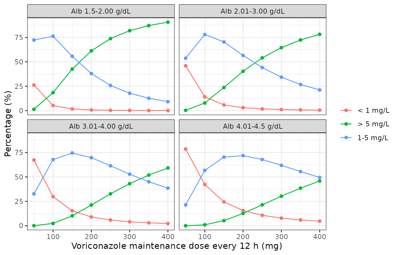
Model counterpart to Figure 3 of Khan-asa 2020 (no omeprazole or omeprazole 20 mg/day): percentage of steady-state troughs in each range by dose and albumin band.
Simulated day-7 profiles and NCA
A virtual cohort of 200 patients per omeprazole group, drawn from the Table 1 albumin distribution, receives the study regimen (400 mg every 12 h for two doses, then 200 mg every 12 h), and is sampled over the day-7 dosing interval as the intensive-sampling patients were.
rxode2::rxSetSeed(20200903)
set.seed(20200903)
n_sub <- 200L

make_arm <- function(n, ome_mgd, id_offset) {
  # Albumin: Table 1 mean 3.04, SD 0.61 g/dL; truncated to the observed
  # 1.6-4.3 g/dL range by redrawing out-of-range values.
  alb <- rnorm(n, 3.04, 0.61)
  while (any(bad <- alb < 1.6 | alb > 4.3)) alb[bad] <- rnorm(sum(bad), 3.04, 0.61)
  tibble::tibble(id = id_offset + seq_len(n), ALB = alb * 10,
                 DOSE_OMEPRAZOLE_MGD = ome_mgd)
}
subj <- dplyr::bind_rows(
  make_arm(n_sub, 0, 0L) |> dplyr::mutate(treatment = "No omeprazole / 20 mg/day"),
  make_arm(n_sub, 40, n_sub) |> dplyr::mutate(treatment = "Omeprazole 40 mg/day")
)

t7 <- 6 * 24 # start of day 7 (first loading dose at time 0)
obs_times <- t7 + c(0, 0.5, 1, 1.5, 2, 3, 4, 6, 8, 10, 12)
doses_df <- dplyr::bind_rows(
  tibble::tibble(time = c(0, 12), amt = 400),
  tibble::tibble(time = seq(24, t7 + 12, by = 12), amt = 200)
) |> dplyr::mutate(evid = 1L, cmt = "depot")
obs_df <- tibble::tibble(time = obs_times, amt = NA_real_, evid = 0L, cmt = "central")
ev <- tidyr::expand_grid(subj, dplyr::bind_rows(doses_df, obs_df)) |>
  dplyr::arrange(id, time, dplyr::desc(evid))

sim <- rxode2::rxSolve(mod, ev, returnType = "data.frame", addDosing = FALSE,
                       keep = "treatment")
#> ℹ parameter labels from comments will be replaced by 'label()'
sim$tad <- sim$time - t7
vpc <- sim |>
  dplyr::group_by(treatment, tad) |>
  dplyr::summarise(p05 = quantile(sim, 0.05), p50 = median(sim),
                   p95 = quantile(sim, 0.95), .groups = "drop")
ggplot(vpc, aes(tad, p50, colour = treatment, fill = treatment)) +
  geom_ribbon(aes(ymin = p05, ymax = p95), alpha = 0.2, colour = NA) +
  geom_line() +
  labs(x = "Time after dose on day 7 (h)", y = "Voriconazole (mg/L)", colour = NULL, fill = NULL) +
  theme_bw()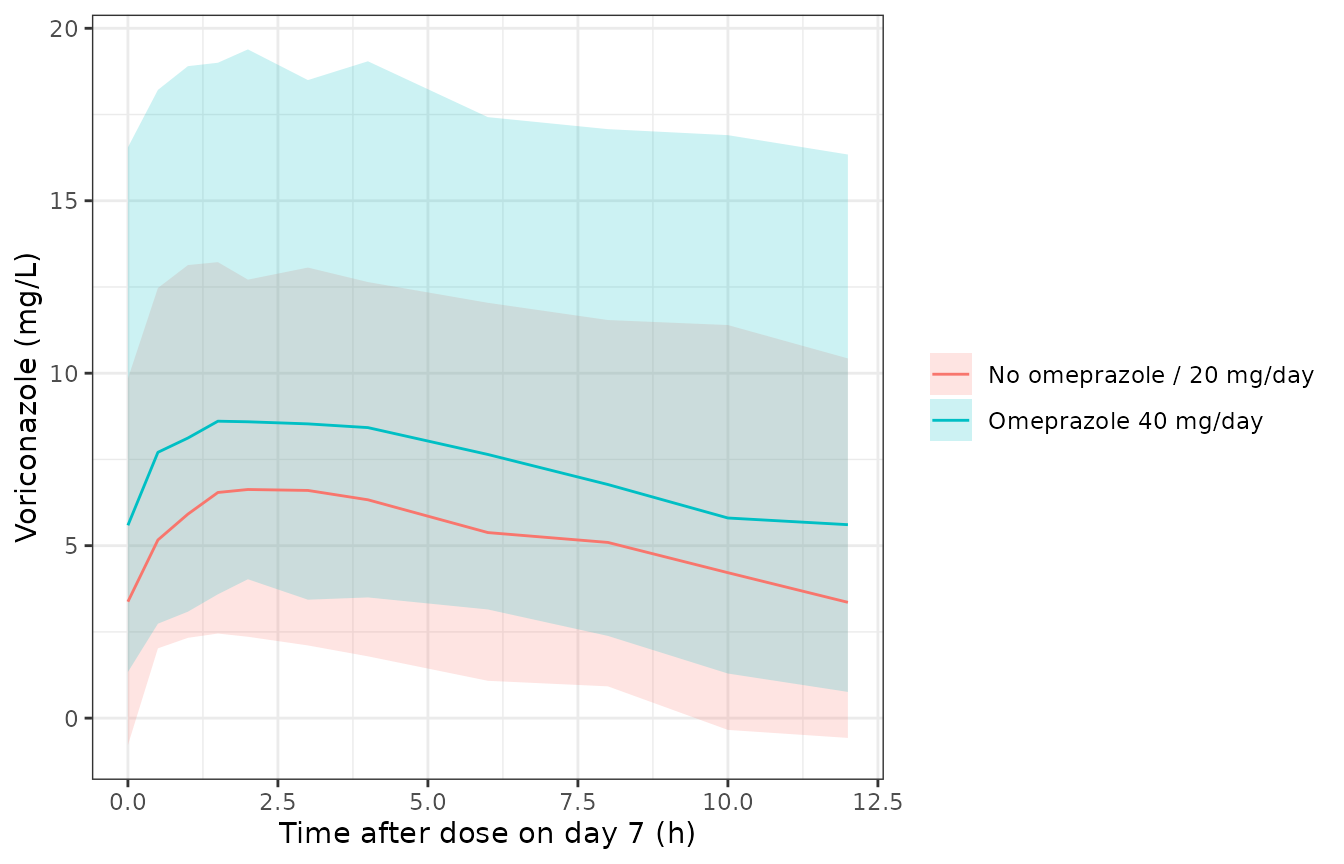
Simulated day-7 voriconazole concentrations (median and 90% interval, with residual error) by omeprazole group.
The paper reports a median observed concentration of 4.49 mg/L, from samples taken at a median of 11.5 h after the dose, pooled over both omeprazole groups. The model’s population median at that time is computed below by the same deterministic quadrature used for the residual-error check (Table 1 albumin distribution, 26% on omeprazole 40 mg/day, clearance eta and additive residual error), so it does not depend on the random cohort. The simulated cohort medians at 12 h are tabulated alongside; the omeprazole 40 mg/day group should sit higher by roughly 1/(1 - 0.306) = 1.44-fold.
mu_115 <- cmin_ss(grid$cl, 11.5)
pop_med <- uniroot(function(q) sum(grid$w * pnorm(q, mu_115, sqrt(2.67))) / sum(grid$w) - 0.5,
                   c(0, 20))$root
cat(sprintf("Model population median at 11.5 h: %.2f mg/L (paper, observed: 4.49 mg/L)\n", pop_med))
#> Model population median at 11.5 h: 4.33 mg/L (paper, observed: 4.49 mg/L)
# Deterministic: a mis-transcribed CL, V or dose moves this by tens of percent.
stopifnot(abs(pop_med / 4.49 - 1) < 0.2)

tr <- sim |>
  dplyr::filter(tad == 12) |>
  dplyr::group_by(treatment) |>
  dplyr::summarise(median_trough = median(Cc), .groups = "drop")
knitr::kable(tr |> dplyr::rename("Group" = treatment, "Median 12-h Cc (mg/L)" = median_trough),
digits = 2)| Group | Median 12-h Cc (mg/L) |
|---|---|
| No omeprazole / 20 mg/day | 3.44 |
| Omeprazole 40 mg/day | 5.35 |
# Robust to the cohort draw: the expected ratio is about 1.44-1.6.
ratio <- tr$median_trough[2] / tr$median_trough[1]
stopifnot(ratio > 1.15, ratio < 2.1)
conc_df <- sim |>
  dplyr::filter(!is.na(Cc)) |>
  dplyr::select(id, treatment, tad, Cc)
dose_df <- subj |>
  dplyr::select(id, treatment) |>
  dplyr::mutate(tad = 0, amt = 200)

conc_obj <- PKNCA::PKNCAconc(conc_df, Cc ~ tad | treatment + id,
                             concu = "mg/L", timeu = "h")
dose_obj <- PKNCA::PKNCAdose(dose_df, amt ~ tad | treatment + id, doseu = "mg")
intervals <- data.frame(start = 0, end = 12, cmax = TRUE, tmax = TRUE,
                        cmin = TRUE, auclast = TRUE, cav = TRUE)
nca <- PKNCA::pk.nca(PKNCA::PKNCAdata(conc_obj, dose_obj, intervals = intervals))
nca_sum <- summary(nca)
knitr::kable(nca_sum, caption = "Simulated day-7 steady-state NCA by omeprazole group.")| Interval Start | Interval End | treatment | N | AUClast (h*mg/L) | Cmax (mg/L) | Cmin (mg/L) | Tmax (h) | Cav (mg/L) |
|---|---|---|---|---|---|---|---|---|
| 0 | 12 | No omeprazole / 20 mg/day | 200 | 61.0 [52.9] | 6.61 [39.7] | 3.30 [83.6] | 2.00 [1.50, 2.00] | 5.09 [52.9] |
| 0 | 12 | Omeprazole 40 mg/day | 200 | 87.2 [51.5] | 8.76 [42.2] | 5.43 [69.1] | 2.00 [2.00, 3.00] | 7.27 [51.5] |
The paper reports no NCA parameters, so there is no published table to compare against. As a consistency check, the median AUCtau in the no-omeprazole group should be close to Dose / typical CL/F = 200 / 3.43 = 58 mg*h/L (the cohort’s mean albumin, 3.04 g/dL, is slightly below the 3.2 g/dL reference, and log-normal clearance makes the median AUC equal to Dose / median CL).
auc_med <- as.data.frame(nca$result) |>
  dplyr::filter(PPTESTCD == "auclast") |>
  dplyr::group_by(treatment) |>
  dplyr::summarise(med = median(PPORRES), .groups = "drop")
auc_med
#> # A tibble: 2 × 2
#>   treatment                   med
#>   <chr>                     <dbl>
#> 1 No omeprazole / 20 mg/day  60.2
#> 2 Omeprazole 40 mg/day       83.9
stopifnot(abs(auc_med$med[1] / (200 / 3.43) - 1) < 0.25)
Assumptions and deviations
-
Residual error scale. Table 2 prints the residual
variability as 2.67 with units mg/L. It is read as the NONMEM
$SIGMAvariance (SD 1.634 mg/L), because the same table reports the IIV as a variance and because Supplementary Figure S1’s lower prediction band is reproduced by SD 1.634 and not by SD 2.67 (see above). The supplementary control stream shows only the base-model$PKblock and does not settle it. -
Omeprazole covariate. The paper’s
OMEindicator is encoded through the daily omeprazole dose columnDOSE_OMEPRAZOLE_MGDwith a 40 mg/day threshold, so that omeprazole 20 mg/day (tested, not retained) carries no effect. Esomeprazole and rabeprazole (3 patients) were not part ofOME. -
Albumin units. The paper’s slope is per g/dL; the
model converts the canonical g/L
ALBcolumn insidemodel(). -
Linear albumin term. The term
1 + 0.249 x (ALB - 3.2)is linear, so it is positive only for albumin above about -0.8 g/dL. It is well defined over the observed 1.6-4.5 g/dL range but should not be extrapolated far outside it. - Virtual cohort. Albumin was drawn from the Table 1 normal distribution (3.04 +/- 0.61 g/dL), redrawn outside the observed range; each omeprazole group was simulated separately with 200 patients.
- Figures 3 and 4. The model reproduces the Section 2.4 worked example (albumin 1.5-2 g/dL, 150 mg) within simulation noise, but not the flatter higher-albumin panels of Figure 3; see the discussion above. No parameter was changed to close that gap.
- Ka. Fixed at 1.1 /h by the authors (from Pascual 2012) because the sparse absorption-phase data could not estimate it; V/F has no IIV for the same reason.