Acetaminophen placental cotyledon perfusion (Mian 2020)
Source:vignettes/articles/Mian_2020_acetaminophen_placentaperfusion.Rmd
Mian_2020_acetaminophen_placentaperfusion.RmdModel and source
Citation: Mian P, Allegaert K, Conings S, Annaert P, Tibboel D, Pfister M, van Calsteren K, van den Anker JN, Dallmann A. Integration of Placental Transfer in a Fetal-Maternal Physiologically Based Pharmacokinetic Model to Characterize Acetaminophen Exposure and Metabolic Clearance in the Fetus. Clin Pharmacokinet. 2020;59(7):911-925. doi:10.1007/s40262-020-00861-7. PMCID: PMC7329787. Perfusion set-up: Section 2.5.1.1; model structure and fixed volumes: Section 2.5.1.2, Figure 3 and Equations 5-8; estimates: Table 1; model fit: Figure 4.
Description: Ex vivo (human term placenta, dual-side recirculating single-cotyledon perfusion). Four-compartment mechanistic model of acetaminophen maternal-to-fetal transfer across an isolated perfused cotyledon: a maternal reservoir and a fetal reservoir, each recirculating through its own half of the cotyledon (maternal and fetal parts), which exchange drug by symmetric passive diffusion (transcotyledon diffusion clearance D_cot) and partition against the perfusate with coefficient K_f,m; a first-order placental elimination K_pe acts on the fetal part. Fitted in MONOLIX to ex vivo perfusion data (Mian 2020 Equations 5-8, Table 1). The paper’s whole-body fetal-maternal PBPK model (MoBi / PK-Sim), into which D_cot and K_f,m were up-scaled, is NOT reproduced here; only the transferable ex vivo placental-transfer model is.
Open-access full text: https://europepmc.org/article/MED/PMC7329787
What this file is, and what it is not
Mian and colleagues built two kinds of model:
| # | Model | Implementation | In this file? |
|---|---|---|---|
| 1 | Ex vivo cotyledon perfusion model (Section 2.5.1.2, Figure 3, Equations 5-8, Table 1) | MONOLIX | yes |
| 2 | Whole-body fetal-maternal PBPK for acetaminophen and its metabolites, with a fetal-liver compartment and three placental-transfer parameterisations (Table 2) | MoBi / PK-Sim | no |
Model 2 extends the authors’ earlier pregnancy PBPK model (Mian et al., Clin Pharmacokinet 2020;59:97-110). Its tissue partition coefficients, organ volumes and blood flows, enzyme reference concentrations and the fetal-liver permeabilities and surface areas are all computed inside the Open Systems Pharmacology software (“automatically estimated using scaling approaches implemented in the software”, Section 2.2) and are not printed in either paper, so it cannot be reconstructed from the publications.
Model 1 is self-contained. It is four ODEs whose rate laws are
printed as Equations 5-8, whose volumes and flows are the stated
experimental settings, and whose three fitted constants are in Table 1.
It is also the part of the paper that transfers: D_cot and
K_f,m are the quantities the authors up-scaled into the
whole-body model (Equation 9), and the ex vivo route was the most
accurate of the three placental-transfer approaches they compared
(Tables 3 and 4).
Population
The model describes an isolated human term placenta, not a patient population. One intact cotyledon per placenta was perfused in a recirculating (closed-closed) dual circuit within 30 min of delivery, with the chorionic artery and vein cannulated (Section 2.5.1.1). Acetaminophen 10 ug/mL – the steady-state concentration at clinical use – was added to the maternal reservoir. Maternal and fetal flows were 14 and 6 mL/min and the mean reservoir volumes 280 and 284 mL. Samples were drawn from both reservoirs at 0, 3, 6, 10, 15, 20 and 30 min, every 15 min to 150 min, then every 30 min to 210 min. The number of placentas perfused is given in the earlier perfusion report (reference 18 of the paper), not in this one.
Source trace
| Quantity | Value | Source |
|---|---|---|
Maternal flow Q_m (q_mat) |
14 mL/min | Section 2.5.1.1 |
Fetal flow Q_f (q_fet) |
6 mL/min | Section 2.5.1.1 |
Maternal reservoir V_m (v_mres) |
280 mL | Section 2.5.1.1 |
Fetal reservoir V_f (v_fres) |
284 mL | Section 2.5.1.1 |
Maternal part of cotyledon V_mp
(v_mcot) |
23 mL, fixed | Section 2.5.1.2 |
Fetal part of cotyledon V_fp (v_fcot) |
35 mL, fixed | Section 2.5.1.2 |
D_cot (ldcot) |
36 mL/min (81%) | Table 1 |
K_pe (lkpe) |
0.0126 1/min (229%) | Table 1 |
K_f,m (lkfm) |
0.737 (35%) | Table 1 |
| Maternal reservoir balance | Equation 5 | Section 2.5.1.2 |
| Maternal cotyledon balance | Equation 6 | Section 2.5.1.2 |
| Fetal cotyledon balance | Equation 7 | Section 2.5.1.2 |
| Fetal reservoir balance | Equation 8 | Section 2.5.1.2 |
| Initial maternal concentration | 10 ug/mL | Section 2.5.1.1 |
| Fitted maternal and fetal curves | read off the figure | Figure 4 |
Simulation
The experiment is one dose of 10 ug/mL x 280 mL = 2800 ug into the maternal reservoir, followed for 210 min.
dose_ug <- 10 * 280
tgrid <- sort(unique(c(seq(0, 210, by = 1), c(3, 6, 10, 15, 20, 30))))
ev <- et(amt = dose_ug, cmt = "maternal_reservoir") |>
  et(tgrid, cmt = "maternal_reservoir")
sim <- as.data.frame(rxSolve(mod, ev))
head(sim[, c("time", "Cmaternal", "Cfetal")])
#>   time Cmaternal     Cfetal
#> 1    0 10.000000 0.00000000
#> 2    1  9.624885 0.01367895
#> 3    2  9.364986 0.06191244
#> 4    3  9.162074 0.13375092
#> 5    4  8.994822 0.21922108
#> 6    5  8.850611 0.31206047
Replicate published figures
Figure 4 of the paper shows the model-predicted maternal and fetal reservoir curves against the ex vivo observations. The two predicted curves were read off the figure by the maintainers at the plotted time points (reading precision about 0.1 ug/mL).
fig4 <- tibble::tribble(
  ~time_h, ~maternal, ~fetal,
  0.05,  8.75, 0.10,
  0.10,  8.40, 0.30,
  0.167, 8.00, 0.62,
  0.25,  7.55, 1.00,
  0.333, 7.20, 1.35,
  0.50,  6.60, 1.90,
  0.75,  5.90, 2.55,
  1.00,  5.40, 3.00,
  1.25,  5.05, 3.30,
  1.50,  4.75, 3.55,
  1.75,  4.58, 3.72,
  2.00,  4.45, 3.83,
  2.25,  4.35, 3.92,
  2.50,  4.28, 3.97,
  3.00,  4.20, 4.04,
  3.50,  4.15, 4.08
) |>
  mutate(time = round(time_h * 60))

ev_fig <- et(amt = dose_ug, cmt = "maternal_reservoir") |>
  et(sort(unique(fig4$time)), cmt = "maternal_reservoir")
sim_fig <- as.data.frame(rxSolve(mod, ev_fig)) |>
  select(time, Cmaternal, Cfetal)

cmp <- fig4 |>
  left_join(sim_fig, by = "time") |>
  mutate(
    pct_maternal = 100 * (Cmaternal - maternal) / maternal,
    pct_fetal = 100 * (Cfetal - fetal) / fetal
  )
cmp |>
  select(time, maternal, Cmaternal, pct_maternal, fetal, Cfetal, pct_fetal) |>
  dplyr::rename(
    "Time (min)" = time,
    "Maternal, Figure 4" = maternal,
    "Maternal, model" = Cmaternal,
    "Maternal diff (%)" = pct_maternal,
    "Fetal, Figure 4" = fetal,
    "Fetal, model" = Cfetal,
    "Fetal diff (%)" = pct_fetal
  ) |>
knitr::kable(digits = 2)| Time (min) | Maternal, Figure 4 | Maternal, model | Maternal diff (%) | Fetal, Figure 4 | Fetal, model | Fetal diff (%) |
|---|---|---|---|---|---|---|
| 3 | 8.75 | 9.16 | 4.71 | 0.10 | 0.13 | 33.75 |
| 6 | 8.40 | 8.72 | 3.83 | 0.30 | 0.41 | 36.14 |
| 10 | 8.00 | 8.28 | 3.56 | 0.62 | 0.79 | 28.05 |
| 15 | 7.55 | 7.82 | 3.62 | 1.00 | 1.24 | 23.60 |
| 20 | 7.20 | 7.42 | 3.04 | 1.35 | 1.63 | 20.40 |
| 30 | 6.60 | 6.75 | 2.22 | 1.90 | 2.27 | 19.27 |
| 45 | 5.90 | 6.00 | 1.72 | 2.55 | 2.96 | 15.99 |
| 60 | 5.40 | 5.48 | 1.53 | 3.00 | 3.42 | 13.95 |
| 75 | 5.05 | 5.12 | 1.33 | 3.30 | 3.72 | 12.78 |
| 90 | 4.75 | 4.86 | 2.26 | 3.55 | 3.92 | 10.35 |
| 105 | 4.58 | 4.67 | 1.96 | 3.72 | 4.04 | 8.61 |
| 120 | 4.45 | 4.53 | 1.82 | 3.83 | 4.11 | 7.40 |
| 135 | 4.35 | 4.43 | 1.74 | 3.92 | 4.15 | 5.93 |
| 150 | 4.28 | 4.34 | 1.48 | 3.97 | 4.17 | 5.00 |
| 180 | 4.20 | 4.22 | 0.50 | 4.04 | 4.16 | 2.94 |
| 210 | 4.15 | 4.13 | -0.48 | 4.08 | 4.12 | 0.98 |
fig4_long <- fig4 |>
  select(time, maternal, fetal) |>
  pivot_longer(-time, names_to = "reservoir", values_to = "conc")
sim_long <- sim |>
  select(time, maternal = Cmaternal, fetal = Cfetal) |>
  pivot_longer(-time, names_to = "reservoir", values_to = "conc")
ggplot() +
  geom_line(data = sim_long, aes(time / 60, conc, colour = reservoir)) +
  geom_point(data = fig4_long, aes(time / 60, conc, colour = reservoir), shape = 1) +
  labs(
    x = "Time (h)", y = "Acetaminophen (ug/mL)", colour = "Reservoir",
    caption = "Replicates Figure 4 of Mian 2020. Lines: this model; circles: the paper's fitted curves read off the figure."
  ) +
  theme_bw()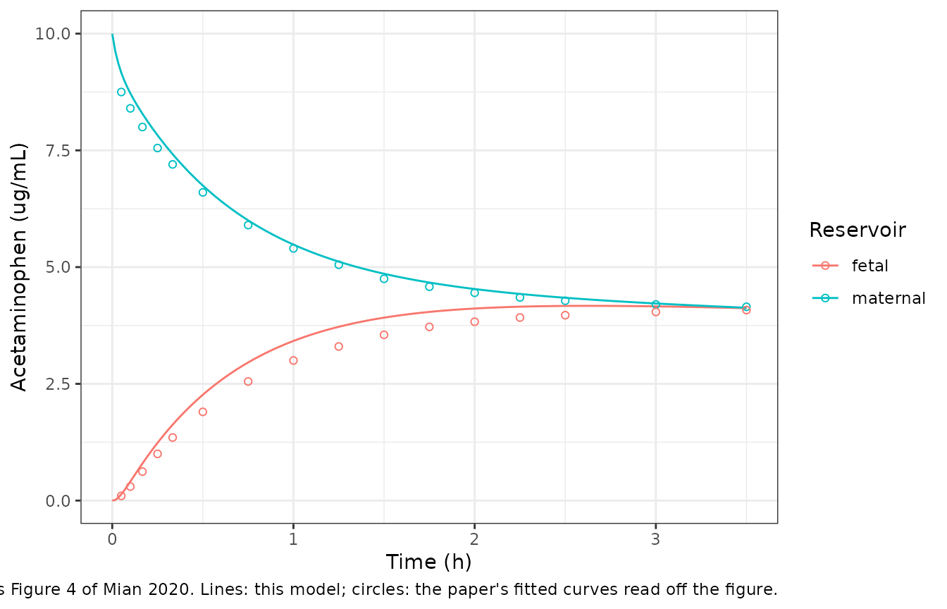
The maternal curve is reproduced within 5% throughout. The fetal curve rises faster than the published one early on – 20-35% above it in the first 20 min, while the fetal concentration is still below 1.5 ug/mL, about 20% at 30 min and 14% at 1 h – and converges on it from 2 h onward (within 1% at 210 min). The published curves are the fit to pooled perfusions – the figure’s own maternal curve starts at 9.5 ug/mL rather than the nominal 10 – whereas this file uses the stated nominal settings, so an early-phase gap of this size is expected; it is not tuned away.
late <- cmp$time >= 60
stopifnot(
  # Maternal decline: a wrong flow, volume or D_cot moves this by tens of %.
  median(abs(cmp$pct_maternal)) < 5,
  max(abs(cmp$pct_maternal)) < 10,
  # Fetal rise: centre within 15%, and within 15% everywhere after 1 h.
  median(abs(cmp$pct_fetal[cmp$time >= 30])) < 15,
  max(abs(cmp$pct_fetal[late])) < 15
)
Structural checks
K_f,m acts on the cotyledon outflows, not on the diffusion step
Equations 5-8 place K_f,m on the flow terms leaving
both halves of the cotyledon (Q_m x C_mp / K_f,m
and Q_f x C_fp / K_f,m), not on the diffusion term between
them. At equilibrium (and ignoring the small K_pe loss)
that makes the two reservoirs equal: Equation 5 gives
C_mp = K_f,m x C_m, Equation 8 gives
C_fp = K_f,m x C_f, and the diffusion term in Equations 6-7
vanishes only when C_mp = C_fp. The Discussion instead
describes K_f,m as “the maternal-to-fetal concentration
ratio at equilibrium”, which would need the partition on the diffusion
step, D_cot x (C_mp - C_fp / K_f,m), and would drive the
fetal:maternal reservoir ratio towards 0.737.
Figure 4 decides between the two. Its fitted curves end at 4.15 (maternal) and 4.08 ug/mL (fetal), a ratio of 0.98, which the printed equations reproduce and the Discussion’s reading does not.
alt <- rxode2({
  Cm <- mres / 280; Cmp <- mcot / 23; Cfp <- fcot / 35; Cf <- fres / 284
  d/dt(mres) <- 14 * Cmp - 14 * Cm
  d/dt(mcot) <- 14 * Cm - 14 * Cmp - 36 * (Cmp - Cfp / 0.737)
  d/dt(fcot) <- 6 * Cf - 6 * Cfp + 36 * (Cmp - Cfp / 0.737) - 0.0126 * 35 * Cfp
  d/dt(fres) <- 6 * Cfp - 6 * Cf
})
ev_end <- et(amt = dose_ug, cmt = "mres") |> et(c(210, 2000), cmt = "mres")
alt_end <- as.data.frame(rxSolve(alt, ev_end))
ev_end_mod <- et(amt = dose_ug, cmt = "maternal_reservoir") |>
  et(c(210, 2000), cmt = "maternal_reservoir")
mod_end <- as.data.frame(rxSolve(mod, ev_end_mod))

ratios <- tibble::tibble(
  Reading = c("Figure 4 (published fit)", "Equations 5-8 as printed", "Partition on the diffusion step"),
  `Fetal:maternal at 210 min` = c(
    4.08 / 4.15,
    mod_end$Cfetal[mod_end$time == 210] / mod_end$Cmaternal[mod_end$time == 210],
    alt_end$Cf[alt_end$time == 210] / alt_end$Cm[alt_end$time == 210]
  )
)
knitr::kable(ratios, digits = 3)| Reading | Fetal:maternal at 210 min |
|---|---|
| Figure 4 (published fit) | 0.983 |
| Equations 5-8 as printed | 0.998 |
| Partition on the diffusion step | 0.738 |
Mass balance and the closed-form equilibrium
With K_pe = 0 the system is closed, so the total amount
must stay at the dose and every compartment must settle where the
partitioning puts it: reservoirs at
D / (V_m + V_f + K_f,m (V_mp + V_fp)) and both cotyledon
halves at K_f,m times that. Both sides of this check use
the same parameters, so a tight bound is correct.
ev_mb <- et(amt = dose_ug, cmt = "maternal_reservoir") |>
  et(c(10, 60, 210, 5000), cmt = "maternal_reservoir")
mb <- as.data.frame(rxSolve(mod, ev_mb, params = c(lkpe = log(1e-12)))) |>
  mutate(total = maternal_reservoir + maternal_cotyledon + fetal_cotyledon + fetal_reservoir)
c_eq <- dose_ug / (280 + 284 + 0.737 * (23 + 35))
mb_end <- mb[mb$time == 5000, ]
stopifnot(
  all(abs(mb$total - dose_ug) / dose_ug < 1e-6),
  abs(mb_end$Cmaternal / c_eq - 1) < 1e-4,
  abs(mb_end$Cfetal / c_eq - 1) < 1e-4,
  abs(mb_end$maternal_cotyledon / 23 / (0.737 * c_eq) - 1) < 1e-4
)
c(closed_form_ug_per_mL = c_eq, simulated_maternal = mb_end$Cmaternal)
#> closed_form_ug_per_mL    simulated_maternal
#>              4.614781              4.614781
Placental elimination over the experiment
K_pe was estimated with a standard error of 229% (Table
1 labels the column “residual standard error”) and the authors called it
“negligibly small” (Section 3.2). Over the 210-min experiment it removes
the following share of the dose:
end210 <- sim[sim$time == 210, ]
lost <- dose_ug - with(end210, maternal_reservoir + maternal_cotyledon + fetal_cotyledon + fetal_reservoir)
pct_lost <- 100 * lost / dose_ug
pct_lost
#> [1] 10.72074
stopifnot(pct_lost > 5, pct_lost < 20)
About a tenth of the dose, so within the experiment K_pe
is small but not negligible; it accounts for the reservoirs ending near
4.1 ug/mL rather than at the closed-system equilibrium of 4.6 ug/mL
computed above. The authors’ judgement concerned the whole-body model,
where K_pe was dropped.
Up-scaling to the whole placenta (Equation 9)
Equation 9 scales the cotyledon clearance to the whole placenta by
volume, D_pl = D_cot x V_pl / V_cot. Table 2 gives
D_pl = 403 mL/min from D_cot = 36 mL/min and
V_cot = 58 mL; the placental volume used is not printed but
follows as
v_pl <- 403 * 58 / 36
v_pl
#> [1] 649.2778
stopifnot(v_pl > 400, v_pl < 900)
about 650 mL, a plausible term placental volume.
NCA
The paper reports no non-compartmental parameters for the ex vivo experiment (the Table 3 NCA values belong to the whole-body PBPK model against in vivo cord-blood data), so there is no published NCA to compare with. For reference, PKNCA summarises the simulated maternal-reservoir decline and the fetal reservoir exposure over the 210-min experiment.
conc <- sim |>
  select(time, Cmaternal, Cfetal) |>
  pivot_longer(-time, names_to = "reservoir", values_to = "conc") |>
  mutate(id = 1L) |>
  filter(!is.na(conc))
dose_df <- tibble::tibble(
  id = 1L, time = 0, amt = dose_ug,
  reservoir = c("Cmaternal", "Cfetal")
)
conc_obj <- PKNCAconc(conc, conc ~ time | reservoir + id)
dose_obj <- PKNCAdose(dose_df, amt ~ time | reservoir + id)
intervals <- data.frame(start = 0, end = 210, cmax = TRUE, tmax = TRUE, auclast = TRUE)
nca <- pk.nca(PKNCAdata(conc_obj, dose_obj, intervals = intervals))
as.data.frame(nca$result) |>
  select(reservoir, PPTESTCD, PPORRES) |>
  pivot_wider(names_from = PPTESTCD, values_from = PPORRES) |>
  dplyr::rename(
    "Reservoir" = reservoir,
    "Cmax (ug/mL)" = cmax,
    "Tmax (min)" = tmax,
    "AUC0-210 (min*ug/mL)" = auclast
  ) |>
knitr::kable(digits = 2)| Reservoir | AUC0-210 (min*ug/mL) | Cmax (ug/mL) | Tmax (min) |
|---|---|---|---|
| Cfetal | 728.58 | 4.17 | 158 |
| Cmaternal | 1100.37 | 10.00 | 0 |
Assumptions and deviations
- Only the ex vivo model is packaged. The whole-body fetal-maternal PBPK model depends on partition coefficients, organ volumes and flows, enzyme reference concentrations and fetal-liver permeabilities that the Open Systems Pharmacology software computes and neither this paper nor its predecessor prints.
-
Equations 5-8 are used as printed. The paper writes
each balance as
dN/dt = (flux terms in N) / V; the right-hand-sideNare read as concentrations and the balances multiplied through byVto give amounts.K_f,mtherefore divides the cotyledon concentration on both the maternal and the fetal outflow. That form makes the reservoirs equilibrate at a fetal:maternal ratio near 1, which disagrees with the Discussion’s wording but matches the paper’s own fitted curves in Figure 4 (see Structural checks). - Nominal starting concentration. The simulation starts the maternal reservoir at the stated 10 ug/mL. Figure 4’s fitted maternal curve starts near 9.5 ug/mL, the likely source of the early fetal difference.
-
K_pe is retained. The authors left
K_peout of the whole-body PBPK model because it was small and imprecise, but it is part of the fitted ex vivo model and is kept here; setlkpeto a very small value to remove it. - No variability. Between-placenta variability and the residual-error model were estimated (Section 2.5.1.2) but their final values are not reported, so the file carries typical values only and has no residual-error lines.
- Metabolites. Acetaminophen-glucuronide and -sulphate transfer were measured in the same perfusions (reference 18) but not modelled in this paper, and are not included.
- Figure 4 values were read off the figure and carry about 0.1 ug/mL of reading error; the observed perfusion concentrations in that figure are not used.